Basics

Introduction

The members of the garnet group have a large variety of chemical compositions with the general formula A²⁺₃B³⁺₂(SiO₄)₃. A is a distorted octahedral site and B a normal octahedral site. Here we focus on the two garnets almandine and andradite, which differ in their chemical composition and the valence state of Fe. Almandine has the chemical formula Fe²⁺₃Al₂(SiO₄)₃, with Fe as Fe²⁺ in the distorted octahedral A site, and andradite has the chemical formula Ca₃Fe³⁺₂(SiO₄)₃, with Fe as Fe³⁺ in the octahedral B site. There is a general, large immiscibility gap between almandine and andradite, however, almandine can have up to ~10% Fe³⁺ and andradite up to ~10% Fe²⁺. This amount is expressed in the atomic ratio Fe³⁺/FeT, with FeT meaning total Fe. The amount of Fe³⁺/FeT can be directly used to calculate the amount of free oxygen, i.e., the oxygen fugacity (\(\rightarrow\) fO₂) while the garnet formed.

Summary

Almandine: Fe²⁺₃Al₂(SiO₄)₃, up to ~10% Fe³⁺/FeT
Andradite: Ca₃Fe³⁺₂(SiO₄)₃, down to ~90% Fe³⁺/FeT
The amount of Fe³⁺/FeT is used to calculate the fO₂.

Principle

The energies of the FeL\(\alpha\) and FeL\(\beta\) lines are close together at 0.7049 and 0.7183 keV, respectively. These energies translate to analyser crystal positions, i.e., L-values on a JEOL microprobe of 191.218 and 187.631 mm. The relative intensities of the lines are 80 and 20, respectively, on a normalised scale of 100. Figure 1 shows the FeLa and FeLb peaks of an almandine spectra. The vertical lines indicate the tabulated values for FeLa and FeLb. A single tabulated and measured values need not to coincide, as this depends on the mechanical build. The distance of FeLa and FeLb, on the other, should be the same between the tabulated and measured peaks. However, this is not the case as already visible in Figure 1 by the naked eye.

Figure 1: An Almandine Fe spectra with the Fe La and Lb lines. Taken with 2 µm steps, 1 s dwell time, 3 accumulations at 100 nA and 15 kV in Diff mode to suppress the FeKa 9. order peak at 189.417 mm (0.7116 keV). Spectra obtained with the GU Frankfurt IfG JEOL EPMA.

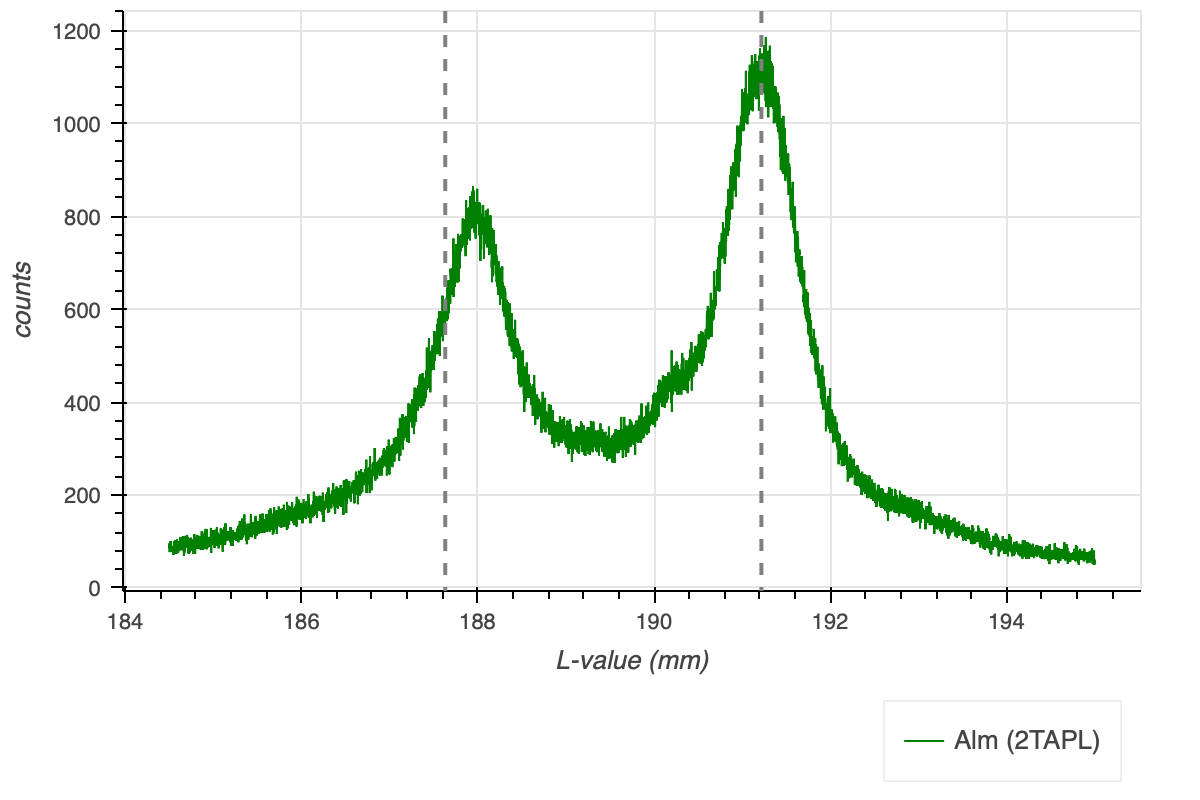
This means, at least one peak is not where it theoretically should be. The reason is the crystal field in which an atom, in this case the Fe atom, sits. This crystal fields slightly changes the electron energy levels around the Fe atom, and therewith the differences between the electron energy levels. Figure 2 illustrates this effect. The lengths of the arrows represent the energy differences when an electron from a higher shell transitions down to a lower shell, thereby emitting the characteristic X-rays with the same energies as these energy difference. The comparison of the arrow lengths on the right illustrate the change in energy difference between the two characteristic lines La and Lb.

Figure 2: Schematic comparison of tabulated Fe energy levels with energy levels that are slightly changed by the crystal field.

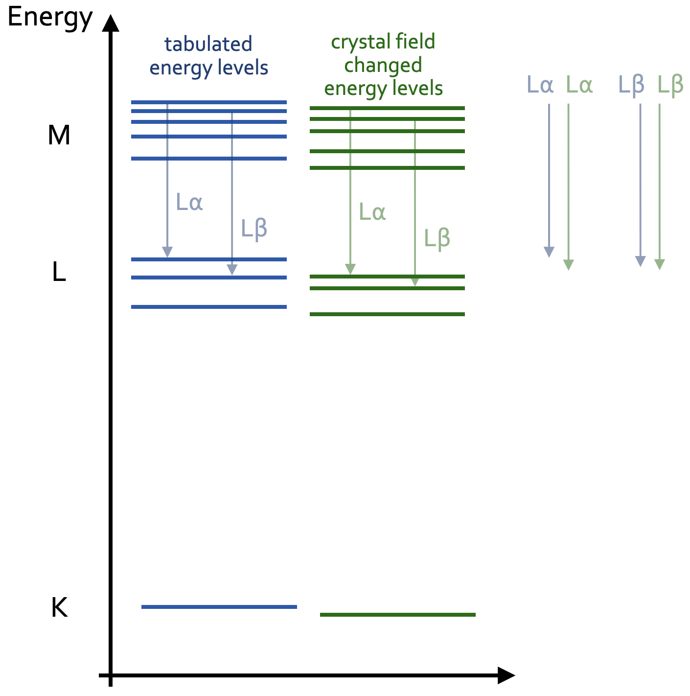
These differences define the energies of the characteristic X-rays of the Lb and La lines. This effect is called chemical peak shift, and is the fundamental effect, upon which the flank method builds. :red[And finally, this effect also changes the relative intensities of the Lb and La lines.]

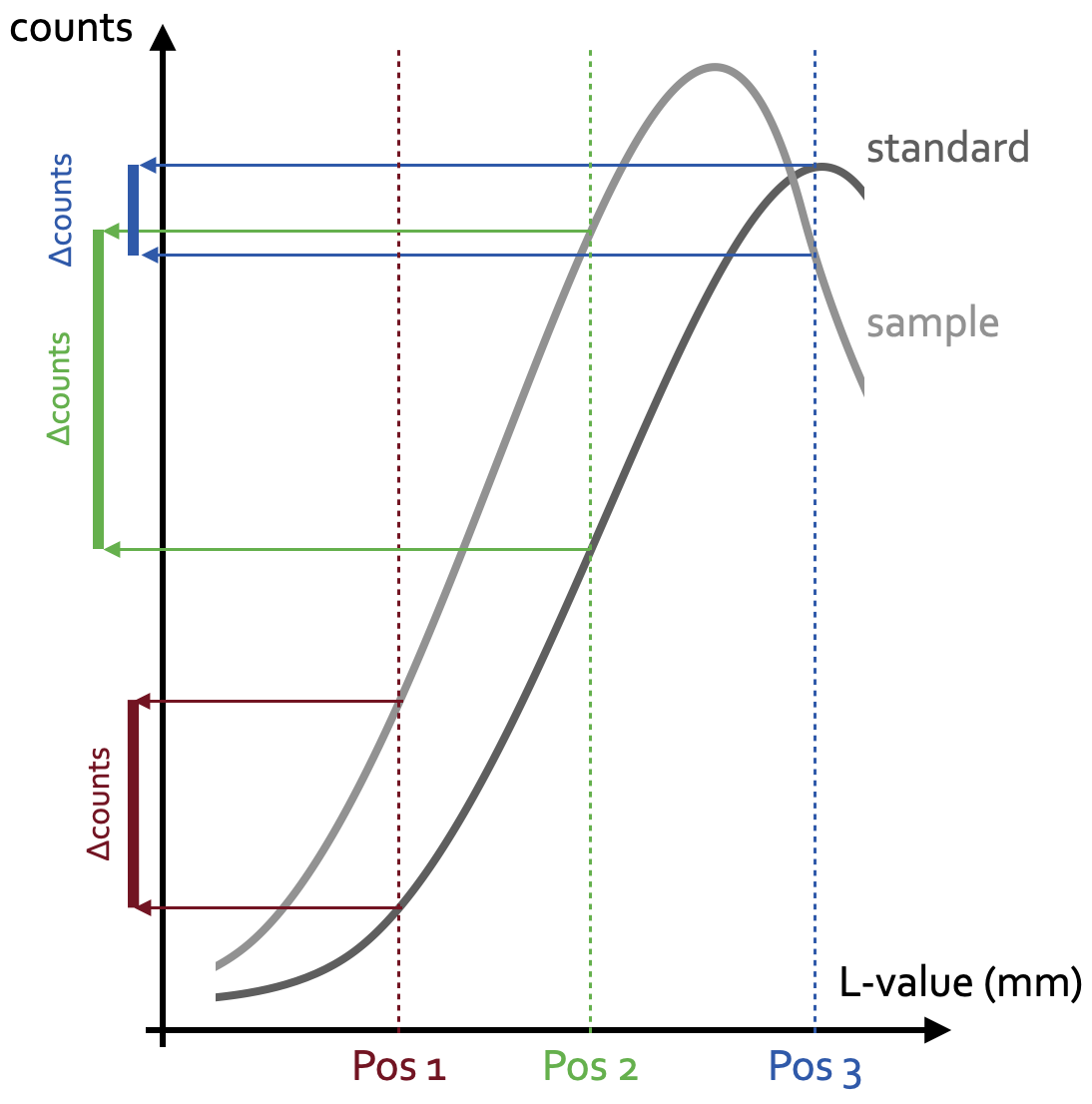
Now, the Fe²⁺ in pure almandine occupies the distorted octahedral site, while the Fe³⁺ in pure andradite occupies the normal octahedral site. These two different crystal fields result in slightly different energy levels, and therewith in different energies of the characteristic La and Lb lines and different peak intensities. Hence, almandine and andradite are discriminated by the location and height of their La and Lb peaks. The goal is, however, not to simply discriminate two minerals, Further, most garnets in mantle and metamorphic rocks are solid solutions between almandine and pyrope with the general formula (Mg,Fe)₃Al₂(SiO₄)₃. These garnets contain, as outlined above, small amounts of Fe³⁺, which is a function of the ambient fO₂ during garnet formation. But even small variations of Fe³⁺ shift the positions and increase/decrease the intensities of the La and Lb peaks. We cannot sensibly quantify an entire spectrum such as the one shown in Figure 1, and obtaining such spectra would cost way too much time. We therefore position the analyser crystal at a certain L-value, and measure the counts at this position in a standard and then in the sample. Because the peak shifted and in- or decreased its intensity depending on the sample’s Fe³⁺/FeT ratio, the counts in the sample will be either lower or higher than in the standard. As these count differences will be small, it is important to move the analyser crystal to a position with maximum count differences between standard and sample. As is seen from the schematic Figure 3, this position is at around the middle of a peak’s flank (now guess how this method earned its name). Each measurement position results in another count difference between the standard and sample peak. Note that peak means somewhere on the peak, not the peak maximum – which would not possible for both peaks at the same time when the measurement position is fixed, but the peak maximum of the samples is shifted from the peak maximum of the standard.

Figure 3: Schematic FeL peak in a standard and a sample. The peak of the sample shifted its position and changed its intensity due to a different amount of Fe³⁺/FeT. Three coloured, dashed, vertical measurement positions (Pos) (\(\rightarrow\) L-values) are indicated.

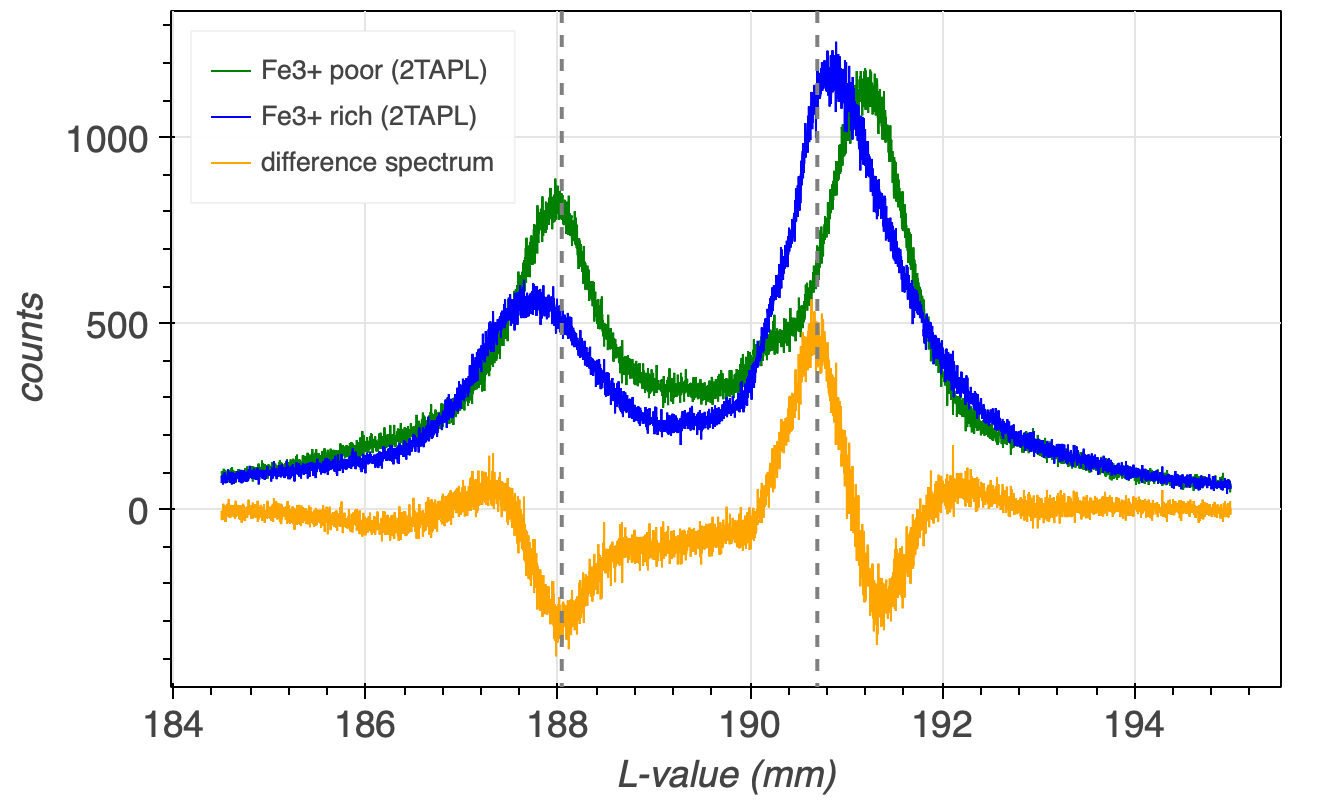
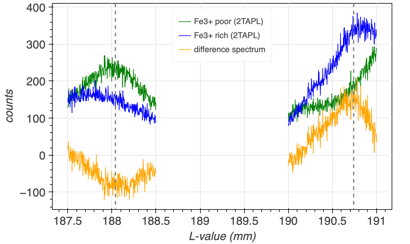
The maximum counts difference between the two spectra can be identified when the counts of spectra, e.g., almandine are subtracted from the counts of the other spectra, which would then be andradite. The positions of the maxima and minima of the resulting difference spectra (orange line in Figure 4) indicate the positions, where the two spectra have their maximum counts differences.

The counts differences between a single, e.g., FeLa standard and sample would insufficiently sensitive to correlate these with Fe³⁺/FeT difference between the standard and the sample. Therefore the counts differences between both, the FeLa and FeLb are determined. To obtain maximum changes in counts, for FeLa the position is chosen, where the difference spectra has its maxima, which will decrease with changing Fe³⁺/FeT, while for FeLb the position is chosen, where the difference spectra has its minima, which will increase with changing Fe³⁺/FeT. The change of counts at these two positions is then expressed by dividing the counts at these two positions, specifically by dividing the counts at the FeLb flank through the counts of the FeLa flank, in short: FeLb/FeLa. This provides a dimensionless number, which is preferable instead of the counts difference, which would be a dimensional number, and depend on measurement conditions.

The two analyser crystal positions should not be too close to their respective peaks, i.e., good analyser crystal positions in case of Figure 4 would be at 188.07 mm for FeLb and at 190.67 for FeLa, as drawn in the figure by the dashed, grey, vertical lines.

Figure 4: FeLa and FeLb spectra for almandine and andradite, and the difference spectra of andradite minus almandine. Dashed, grey, vertical lines indicate ideal measurement positions for the TAPL analyser crystal positions. Measurement conditions are the same as for Figure 1.

Summary

Fe³⁺/FeT-poor (e.g., almandine) and Fe³⁺/FeT-rich (andradite) garnets have different chemical peak shifts. The extent of this chemical peak shift is a function of the garnet’s Fe³⁺/FeT and FeT. Count rates are measured on the FeLa and FeLb flanks and from these the dimensionless FeLb/FeLa-ratio is calculated. This ratio together with the FeT of a granet is used to determine its Fe³⁺/FeT.

Application

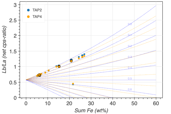
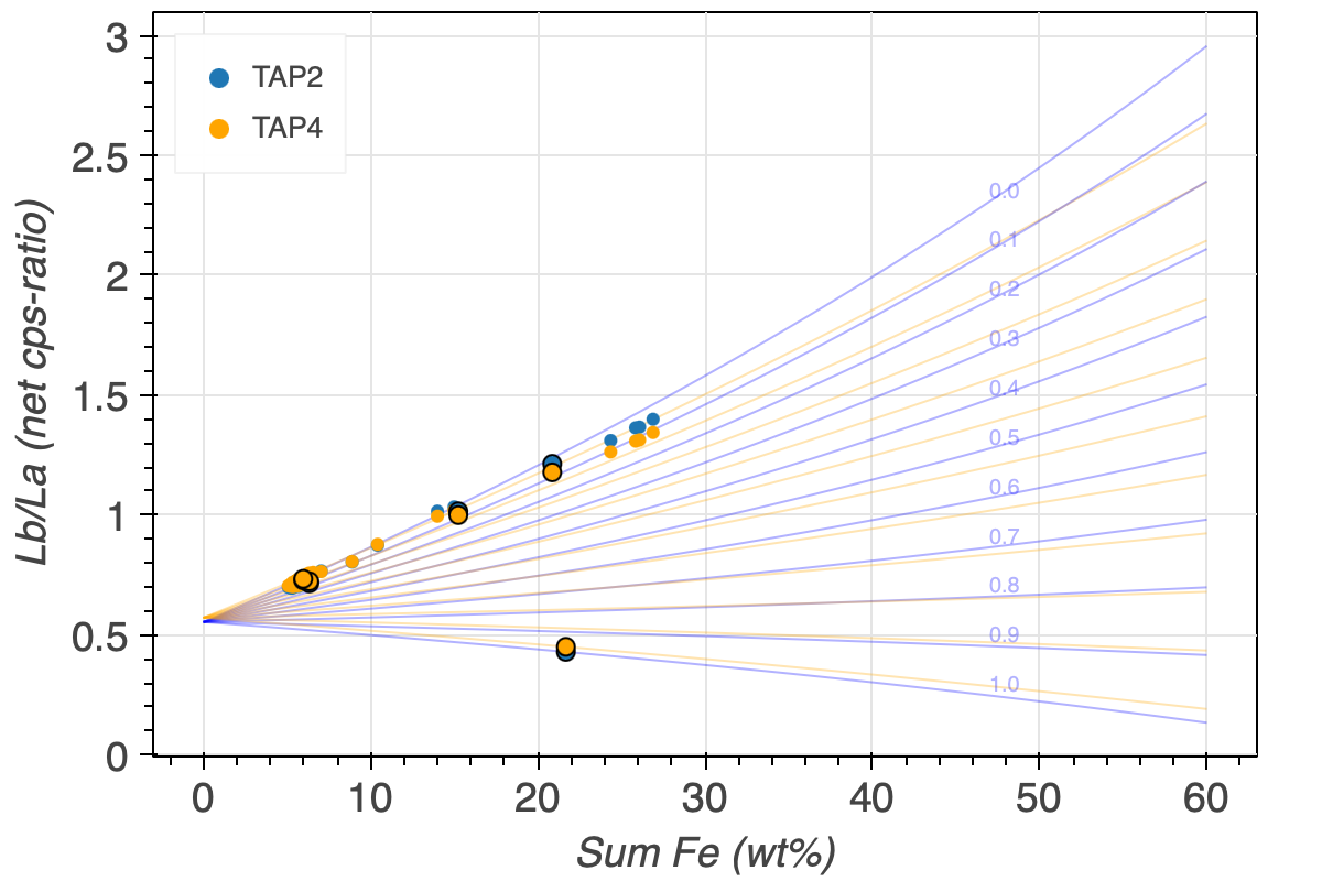
The FeLb/FeLa of a garnet not only depends on its Fe³⁺/FeT, but also on its Fe-content. Figure 5 illustrates this dependency, with the total Fe on the x/ and the FeLb/FeLa ratio on the y-axis. Standards with an ideally wide range of FeT concentrations are therefore imperative. This parametrisation plot and how it is calculated is explained in the next section.

The spread of the iso-Fe³⁺/FeT lines depends on the chosen standards. If only Fe³⁺/FeT-poor garnets are chosen (Figure 5 (a)), the spread is large, and the resolution, i.e., the precision of the Fe³⁺/FeT becomes better. The addition of an andradite standard decreases the spread of the iso-Fe³⁺/FeT lines, and reduces the Fe³⁺/FeT resolution (Figure 5 (b)). Finally, the precision of determining the Fe³⁺/FeT becomes increasingly better with increasing FeT, which correlates with a significant increase in the iso-Fe³⁺/FeT lines spread. And vice versa, the lower the FeT in garnet, the more imprecise it becomes to determine its iso-Fe³⁺/FeT.

(a) Only pyrope-alamandine standards

(b) Almandine and one andradite standard

Figure 5: The FeLb/FeLa ratio depends on the Fe³⁺/FeT and the FeT concentration of a garnet. The blue and orange lines represent lines of the same Fe³⁺/FeT content, with high FeLb/FeLa represent high Fe³⁺/FeT and vice versa. Standards: large, black-rimmed symbols. Samples: small symbols.

Parametrisation

Regression formulas, in which the parameters are used:

\(Fe^{2+} = A + B \times \frac{L\beta}{L\alpha} + C \times \Sigma Fe + D \times \Sigma Fe \times \frac{L\beta}{L\alpha}\)

\(Fe^{3+} = -A - B \times \frac{L\beta}{L\alpha} - C \times \Sigma Fe - D \times \Sigma Fe \times \frac{L\beta}{L\alpha} + Fe_{tot}\)

x = \(L\beta/L\alpha\)
y = \(Fe_{tot}\)
z = \(Fe^{2+}\)

A = [
[n, \(\Sigma x\), \(\Sigma y\), \(\Sigma(x \times y)\)],
[\(\Sigma x\), \(\Sigma x^2\), \(\Sigma(x \times y)\), \(\Sigma (y \times x^2)\)],
[\(\Sigma y\), \(\Sigma(x \times y)\), \(\Sigma(y^2)\), \(\Sigma(x \times y^ 2)\)],
[\((x \times y)\), \(\Sigma((x^2) \times y)\),
\(\Sigma(x \times y^2)\), \(\Sigma((x^2) \times (y^2)\)]
]

v = [\(z\), \(\Sigma(z \times x)\), \(\Sigma(z \times y)\), \(\Sigma(x \times y \times z)\)]

regression parameters:
rfp = np.linalg.inv(A) @ v

res = rfp[0] + rfp[1] * \(L\beta/L\alpha\) + rfp[2] * \(Fe_{tot}\) + rfp[3] * (\(Fe_{tot}\) * \(L\beta/L\alpha\))

resultsFe3FP = (\(Fe_{tot}\) - res)/\(Fe_{tot}\)

Conclusion

The flank method is an elegant, cost efficient high resolution technique to determine Fe³⁺/FeT, and at the same time the chemical composition of the garnet. It has the potential to be used in a wide range of minerals. The main drawback is the tedious effort to setup the flank method for a new mineral type, which requires a range of minerals with variable FeO-concentrations and known Fe³⁺/FeT, as e.g., determined using Mössbauer quadrupole splitting.

Alternatives

Alternative methods to determine Fe³⁺/FeT are Mössbauer spectroscopy or XANES (X-ray absorption near edge structure). Mössbauer spectroscopy has a low resolution in the typical range of tens of µm, while XANES requires a synchrotron and is therefore costly and laborious. These methods can, however, determine Fe³⁺/FeT in basically all types of material.

Determining Analyser Crystal Positions

The flank method requires measurements on the FeLa and FeLb flanks rather than on their respective peaks. The ideal positions of the analyser crystals are best determined using a difference spectra, as described in the previous section. For garnet, this is best produced from a qualitative almandine and and andradite scan. It is, however, not required to record full spectra, as small intervals across the expected minima and maxima of the difference spectra are sufficient. Sufficient step size and dwell time – i.e., the counting time at each step – can be comparatively small, e.g., a step size of 3 µm and a dwell time of 300 ms. Figure 6 shows such segmented spectra with an interval for FeLa from 187.5 to 188. 5 mm, and for FeLb from 190 to 191 mm, as well as the resulting difference spectra. A high current of e.g., 300 nA is advisable, to obtain higher count rates. The sole measurement time will then be approx. 7 min, i.e., recording the required spectra should take about 10 min, if predefined measurement recipes are used.

Figure 6: A segmented Fe spectra for fast determination of the FeLa and FeLb analyser crystal positions.

The flank data reduction program has a tool to determine analyser crystal positions (‘Crystal Positioning’ in ‘Tools’). Figure 7 shows how a csv table needs to be prepared for this tool. The ‘Datasets’ section further provides a test dataset for download that also serves as a template.

Figure 7: Required header row and layout for csv tables to be used with the crystal positioning tool of the data reduction program.

Summary

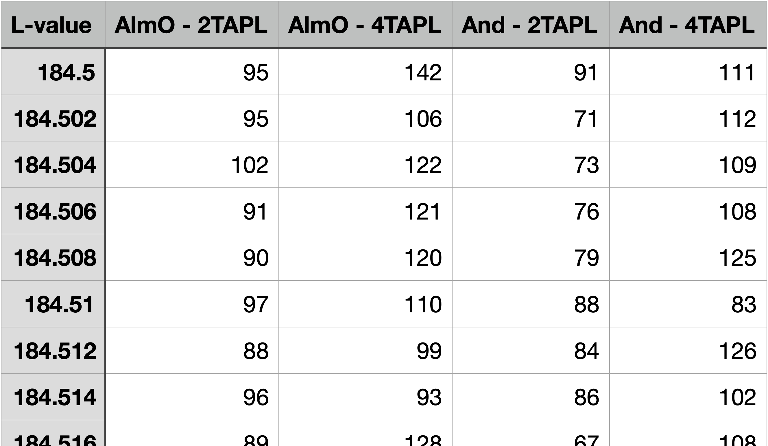
Segmented Fe spectra are sufficient to determine analyser crystal positions, e.g., using the one from the Tools section in the data reduction program.

EPMA Set-Up

The flank method requires measuring the FeLa, FeLb flanks, as well as the Fe-concentration, e.g., on FeKa. The FeLa and FeLb flank measurement positions need to be input manually, after these have been determined as described above. The flank measurement set-ups in the EPMA measurement program might be labelled with element names that are never or only very rarely used. For the FeLb line, this could be Bi or Br and vor La Ar or As.

The FeLa and FeLb lines can be measured using a TAP-crystal, ideally a large-type TAPL cyrstal for better count rates, as the Fe L-lines are comparatively weak. Figure 8 shows a possible EPMA flank measurement set-up, in which the FeLa and FeLb lines are measured using the TAPL crystal of spectrometer 2 (2TAPL), and redundantly also on 4TAPL, to validate the results obtained with 2TAPL (or vice versa).

Figure 8: The EPMA-measurement program and set-up for the FeLa and FeLb flanks. The flanks are measured on 2 spectrometers for cross-validation.

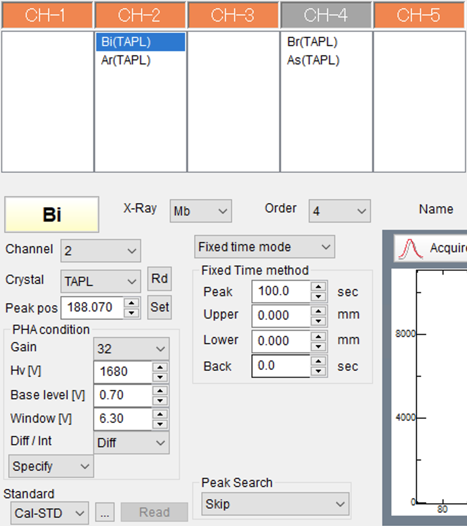
The selected Bi in Figure 8 represents the FeLb flank. The X-ray line as well as the order are as random as the selected Bi for labelling the measurement conditions of the actual FeLb line that is measured with this set-up. The peak position is input manually as determined using e.g., the data reduction program crystal positioning tool. The PHA conditions are determined as usual. The measurement time on all flanks is 100 s. No backgrounds are measured, i.e., the net count rates will be used to determine Fe³⁺ abundances.

The remaining spectrometers can be used for normal element analyses. Measuring Fe is mandatory, as it is required to determine Fe³⁺ abundances. It is, hence, also mandatory to at least measure all main elements, as these are required for accurate matrix corrected Fe concentrations. As the measurement of the flanks takes a little longer than 200 s (considering movement times of the analyser crystals), there might be time for further elements. Figure 9 displays a measurement set-up frequently used at the Institut für Geowissenschaften JEOL EPMA at the Goethe Universität Frankfurt.

Figure 9: A full IfG GU Frankfurt EPMA flank measurement set-up.

Summary

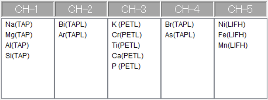
The FeLa & FeLb measurement set-ups are labelled with fake elements, and measured for cross-validation on two spectrometers using TAPL crystals. Fe and main elements need to be measured for accurate Fe concentrations, further elements can be added.