pip install mag4Requirement already satisfied: mag4 in /Users/dominik/anaconda3/lib/python3.11/site-packages (0.0.214)
Note: you may need to restart the kernel to use updated packages.Ein unbekannter Datensatz kann mit einigen wenigen Methoden in pandas statistisch beschrieben werden. Datensätze enthalten häufig Zeilen, Spalten oder Zellen ohne Werte, die manchmal gelöscht werden sollen. pandas erlaubt ein schnelles Daten cleanup, um entsprechende Spalten/Zeilen zu löschen. Schließlich werden Ausreißer in Datensätzen identifiziert und dargestellt.
.describe(), .dropna(), .interpolate()
Die typischen statistischen Beschreibungen eines Datensatzes wie min/max Werte, Mittelwert, Standardawbweichung etc. werden mit .describe aufgerufen. Mit .dropna() werden unerwünschte Zeilen und Spalten eines Datensatzes gelöscht, und mit .interpolate() können Zellen ohne Werte um berechnete Werte ergänzt werden.
.rolling()
Mit .rolling() wird ein gleitender Mittelwert, eine gleitende Summe, etc. eines Datensatzes berechnet, der umgehend dargestellt werden kann.
import mag4 as mg
import pandas as pd
import numpy as np
import matplotlib.pyplot as plt
df = pd.DataFrame(np.random.rand(100))df.rolling(window=5).mean()| 0 | |
|---|---|
| 0 | NaN |
| 1 | NaN |
| 2 | NaN |
| 3 | NaN |
| 4 | 0.317507 |
| ... | ... |
| 95 | 0.562846 |
| 96 | 0.661084 |
| 97 | 0.746175 |
| 98 | 0.725283 |
| 99 | 0.727208 |
100 rows × 1 columns
plt.plot(df)
plt.plot(df.rolling(window=30).mean())
plt.axhline(df.mean().values, color='g')
plt.axhline(df.mean().values + df.std().values, color='y', linestyle='--')
plt.axhline(df.mean().values - df.std().values, color='y', linestyle='--')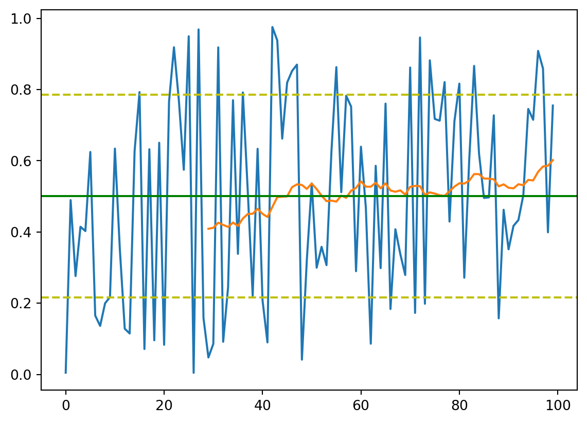
df = pd.read_csv('https://storage.googleapis.com/berkeley-earth-temperature-hr/global/Land_TAVG_monthly.txt', sep='\s+', comment='%', usecols=[0,1,2,3], names=['Year', 'Month', 'Anomaly', 'Unc.'])df.describe().round(2)| Year | Month | Anomaly | Unc. | |
|---|---|---|---|---|
| count | 3305.00 | 3305.00 | 3305.00 | 3305.00 |
| mean | 1887.21 | 6.49 | -0.18 | 0.65 |
| std | 79.52 | 3.45 | 0.63 | 0.52 |
| min | 1750.00 | 1.00 | -2.66 | 0.03 |
| 25% | 1818.00 | 3.00 | -0.57 | 0.16 |
| 50% | 1887.00 | 6.00 | -0.22 | 0.53 |
| 75% | 1956.00 | 9.00 | 0.13 | 1.03 |
| max | 2025.00 | 12.00 | 2.32 | 2.70 |
win_width = 30
plt.plot(df['Year'], (df['Anomaly']+df['Unc.']).rolling(window=win_width).mean(), color='y', linestyle='--')
plt.plot(df['Year'], (df['Anomaly']-df['Unc.']).rolling(window=win_width).mean(), color='y', linestyle='--')
# plt.plot(df['Year'], df['Anomaly'])
plt.plot(df['Year'], df['Anomaly'].rolling(window=win_width).mean())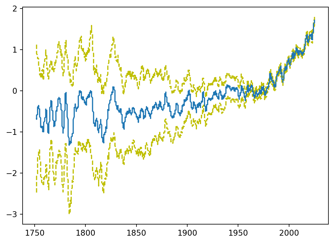
df = mg.get_data('Banda Arc')df['Mg'].mean(), df['Mg'].std()(29792.89462295082, 47804.12174784328).quantile(), .boxplot()
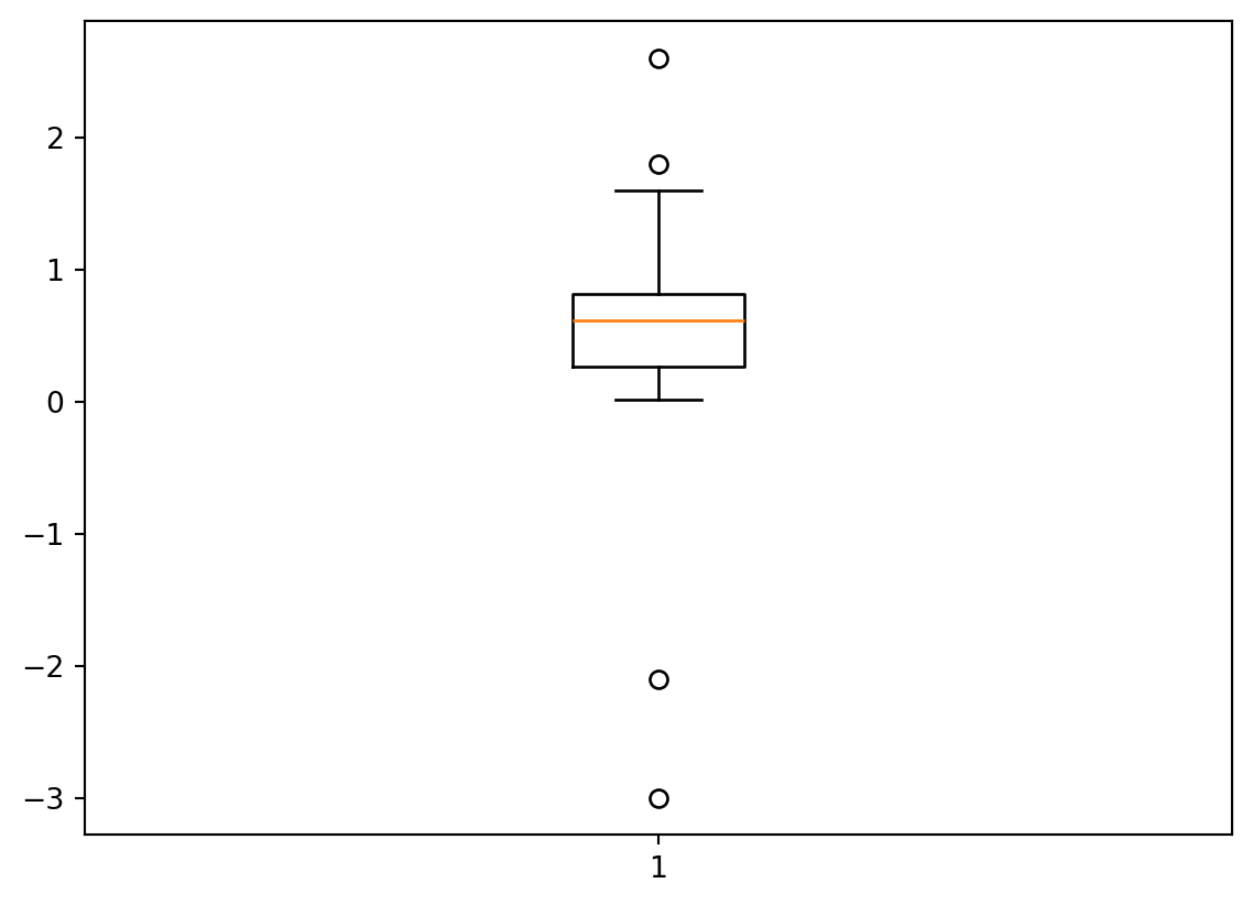
Wir lernen 2 Definitionen für Ausreißer kennen, die wir selbst berechnen und dabei .quantile() kennen lernen. Ausreißer lassen wir dann automatisch in einem Boxplot mit .boxplot()darstellen.
import mag4 as mg
import pandas as pd
import numpy as np
import matplotlib.pyplot as plt
df = pd.DataFrame(np.concatenate([np.random.rand(100), [1.6, 1.8, -2.1, -3, 2.6]]))df.describe()| 0 | |
|---|---|
| count | 105.000000 |
| mean | 0.524557 |
| std | 0.583080 |
| min | -3.000000 |
| 25% | 0.265453 |
| 50% | 0.612338 |
| 75% | 0.810928 |
| max | 2.600000 |
df_out = (df[0] - df[0].mean()) / df[0].std()
fil = (df_out >= 3) | (df_out <= -3)
df[fil]| 0 | |
|---|---|
| 102 | -2.1 |
| 103 | -3.0 |
| 104 | 2.6 |
iqr = df[0].quantile(.75) - df[0].quantile(.25)
df[0].quantile(.25) - 1.5 * iqr, df[0].quantile(.75) + 1.5 * iqr
(-0.5527604967137063, 1.629141569514991)df[0].quantile(.25) - 1.5 * iqr, df[0].quantile(.75) + 1.5 * iqr
fil = (df[0] >= df[0].quantile(.75) + 1.5 * iqr) | (df[0] <= df[0].quantile(.25) - 1.5 * iqr)
df[fil]| 0 | |
|---|---|
| 101 | 1.8 |
| 102 | -2.1 |
| 103 | -3.0 |
| 104 | 2.6 |
plt.axhline(df[0].mean(), color='orange')
plt.axhline(df[0].mean() + df[0].std(), color='y', linestyle='--')
plt.axhline(df[0].mean() + 3*df[0].std(), color='lightgrey', linestyle='--')
plt.axhline(df[0].mean() - df[0].std(), color='y', linestyle='--')
plt.axhline(df[0].mean() - 3*df[0].std(), color='lightgrey', linestyle='--')
plt.scatter(range(105), df)
plt.scatter(range(len(df[fil])), df[fil])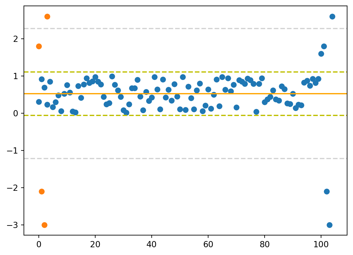
plt.boxplot(df[0]){'whiskers': [<matplotlib.lines.Line2D at 0x177059190>,
<matplotlib.lines.Line2D at 0x177059ad0>],
'caps': [<matplotlib.lines.Line2D at 0x17705a4d0>,
<matplotlib.lines.Line2D at 0x17705ab90>],
'boxes': [<matplotlib.lines.Line2D at 0x177058790>],
'medians': [<matplotlib.lines.Line2D at 0x17705b390>],
'fliers': [<matplotlib.lines.Line2D at 0x17705bc90>],
'means': []}