pip install mag45 Komplexeres Plotten & Statistik I [57:38]
In dieser letzten Einheit Daten darzustellen zeige ich – ansatzweise – wie vielfältig mit Jupyter Notebooks, bzw. Python geplottet werden kann, bzw. wie enorm flexibel interaktive Elemente genutzt werden können. Mit dem Package ›geopandas‹ lernen wir außerdem die Möglichkeit kennen, Daten auf Karten darzustellen – natürlich geht auch das interaktiv. Die Bedeutung guter, aussagekräftiger, übersichtlicher, und dabei durchaus komplexer Diagramme kann nicht ausreichend unterstrichen werden. Diagramme und Abbildungen bilden fast immer den Kern eines sehr guten papers, Vortrags oder natürlich einer Abschlussarbeit. Das gelingt jedoch nur mit dem entsprechenden Werkzeug. Matplotlib gehört sicherlich zu den besten Werkzeugen, um wissenschaftliche Diagramme und Abbildungen zu erzeugen. Die hohe Flexibilität interaktiver Elemente erlaubt es sehr schnell und übersichtlich Daten zusammen mit anderen Daten unterschiedlichster Quellen und beliebiger Menge zu visualisieren und analysieren. Das ist ein sehr guter, erster Schritt, um Daten zu verstehen, um dann in die Detail-Analyse zu gehen.
5.2 Program- Advanced matplotlib plotting [18:30]
fig, ax, subplots(), .subplots_adjust(hspace = 0, wspace = 0), sharex, .set(xlabel = ), .xaxis.set_ticks_position(›both‹), .minorticks_on(), .tick_params(which = ›major‹, length = 7, width = 1, direction = ›in‹), .savefig()
Verwende wie in 5.2 mag4, um Datein zu einzulesen
Jupyter Notebooks, bzw. Python können sehr gut verwendet werden um sehr gute, das bedeutet, sehr übersichtlich, aussagekräftige, und dabei auch komplexe Plots zu erstellen. Es ist praktisch alles möglich – wie meist bei Programmierung –, die Frage ist daher selten ob etwas geht, sondern nur wie das Gewünschte geht. Ich zeige hier ein paar wesentliche Möglichkeiten, welche häufig und typischer für die Mineralogie sind, und verweise sonst auf die tatsächlich diese Woche überarbeitete Dokumentationsseite von https://matplotlib.org, welche mit der Überarbeitung deutlich übersichtlicher und hilfreicher geworden ist (sieht also anders aus als im eben erst erstellten Video). Es lohnt sich schon deshalb, die Seite einmal zu besuchen, um zu sehen, was alles an Diagrammen überhaupt möglich ist. Außerdem zeige ich den Befehl, wie erstellte Abbildungen gespeichert werden können.
Video nb
pip install mag4import mag4 as mg
import matplotlib.pyplot as plt
df = mg.available_datasets()
df| dois | Upload Date | Name | Description | Version | Licence | Keywords | Type | Comments | Short Title | Comment | ORCID | Creation Date | References | Title | Request doi | Source | |
|---|---|---|---|---|---|---|---|---|---|---|---|---|---|---|---|---|---|
| 0 | NaN | 21.01.2024 | Dominik Hezel | xxx | NaN | CC-BY-SA | xxx | Database Dataset | NaN | eastsearid | NaN | 0000-0002-5059-2281 | NaN | NaN | Easter Seamount Chain Salas Y Gomez Ridge | NaN | Georoc |
| 1 | NaN | 21.01.2024 | Dominik Hezel | xxx | NaN | CC-BY-SA | xxx | basic | NaN | chondprop | NaN | 0000-0002-5059-2281 | NaN | NaN | Chondrite Properties | NaN | NaN |
| 2 | NaN | 2025-05-16 | Dominik C. Hezel | example dataset | NaN | CCO | chondrules, Fe, isotopes, example data | Example | NaN | chdfeisoexdat | NaN | https://orcid.org/0000-0002-5059-2281 | NaN | NaN | chondrule Fe isotope example data | no | NaN |
| 3 | NaN | 21.01.2024 | Dominik Hezel | xxx | NaN | CC-BY-SA | xxx | basic | NaN | chemelprop | NaN | 0000-0002-5059-2281 | NaN | NaN | Chemical Element Properties | NaN | NaN |
| 4 | NaN | 21.01.2024 | Dominik Hezel | xxx | NaN | CC-BY-SA | xxx | Database Dataset | NaN | bastcrat | NaN | 0000-0002-5059-2281 | NaN | NaN | Bastar Craton | NaN | Georoc |
| 5 | NaN | 2024-02-06 | Dominik Hezel | Basic data of nuclides | v1.0 | CCO | nuclides, half-lifes, binding-energies | Basic | NaN | nucbasics | NaN | https://orcid.org/0000-0002-5059-2281 | 2024-02-06 | NaN | nuclides-basics | NaN | IAEA - Nuclear Data Section |
| 6 | NaN | 21.01.2024 | Dominik Hezel | xxx | NaN | CC-BY-SA | xxx | Database Dataset | NaN | ninetyrid | NaN | NaN | NaN | NaN | Ninetyeast Ridge | NaN | Georoc |
| 7 | NaN | 2025-03-14 | Lara Friedrichs | In this table the main elements of the sun's p... | NaN | CC-BY SA | elements, sun, photosphere | Basic | NaN | elements photosphere sun | NaN | https://orcid.org/0009-0001-7264-5081 | 2025-03-14 | NaN | test_table_elements | no | Lodders, K., & Fegley, B. (1998). The planetar... |
| 8 | NaN | 2025-05-19 | Dominik C. Hezel | a brief list of mineral compositions | NaN | CCO | mineral data, example | Basic | NaN | mineraldatex2 | NaN | https://orcid.org/0000-0002-5059-2281 | NaN | NaN | Mineral Data Example Dataset 2 | no | NaN |
| 9 | NaN | 21.01.2024 | Dominik Hezel | xxx | NaN | CC-BY-SA | xxx | Database Dataset | NaN | emei | NaN | 0000-0002-5059-2281 | NaN | NaN | Emeishan | NaN | Georoc |
| 10 | NaN | 21.01.2024 | Dominik Hezel | xxx | NaN | CC-BY-SA | xxx | Database Dataset | NaN | mcdis | NaN | 0000-0002-5059-2281 | NaN | NaN | McDonald Islands | NaN | Georoc |
| 11 | NaN | 21.01.2024 | Dominik Hezel | xxx | NaN | CC-BY-SA | xxx | Database Dataset | NaN | namcord | NaN | 0000-0002-5059-2281 | NaN | NaN | North American Cordillera - Paleozoic | NaN | Georoc |
| 12 | NaN | 21.01.2024 | Dominik Hezel | xxx | NaN | CC-BY-SA | xxx | basic | NaN | etransenergies | NaN | 0000-0002-5059-2281 | NaN | NaN | Element Electron Transition Energies | NaN | NaN |
| 13 | NaN | 21.01.2024 | Dominik Hezel | xxx | NaN | CC-BY-SA | xxx | basic | NaN | chondelab | NaN | 0000-0002-5059-2281 | NaN | NaN | Chondrite Element Abundances | NaN | NaN |
| 14 | NaN | 2025-06-24 | Dominik C. Hezel | movement data for the San Andreas fault in cm | NaN | CCO | creep data | Example | NaN | sanancreep | NaN | https://orcid.org/0000-0002-5059-2281 | NaN | NaN | San Andreas creep | no | NaN |
| 15 | NaN | 21.01.2024 | Dominik Hezel | xxx | NaN | CC-BY-SA | xxx | Database Dataset | NaN | karaf | NaN | 0000-0002-5059-2281 | NaN | NaN | Karoo Province - Africa | NaN | Georoc |
| 16 | NaN | 2025-05-19 | Dominik C. Hezel | a brief list of mineral compositions | NaN | CCO | mineral data, example | Example | NaN | mineraldatex | NaN | https://orcid.org/0000-0002-5059-2281 | NaN | NaN | Mineral Data Example Dataset | no | NaN |
| 17 | NaN | 21.01.2024 | Dominik Hezel | xxx | NaN | CC-BY-SA | xxx | basic | NaN | ebindenergies | NaN | 0000-0002-5059-2281 | NaN | NaN | Element Electron Binding Energies | NaN | NaN |
| 18 | NaN | 21.01.2024 | Dominik Hezel | xxx | NaN | CC-BY-SA | xxx | Database Dataset | NaN | galis | NaN | 0000-0002-5059-2281 | NaN | NaN | Galapagos Islands | NaN | Georoc |
| 19 | https://doi.org/10.1180/mgm.2021.43 | 09.12.2023 | Dominik Hezel | IMA–CNMNC approved mineral symbols | NaN | CC-BY-SA | xxx | basic | NaN | abminsym | Another string with\n multiple\n line breaks. | 0000-0002-5059-2281 | 08.06.2021 | Warr LN (2021) Mineralogical Magazine, 85:3, 2... | Abbreviated Mineral Symbols | NaN | paper supplement by L. N. Warr |
| 20 | NaN | 21.01.2024 | Dominik Hezel | xxx | NaN | CC-BY-SA | xxx | Database Dataset | NaN | hybibplat | NaN | 0000-0002-5059-2281 | NaN | NaN | Hyblean or Iblean Plateau, Sicily | NaN | Georoc |
| 21 | NaN | 2025-05-19 | Dominik C. Hezel | a brief list of mineral compositions | NaN | CCO | mineral data, example | Example | NaN | mineraldatex3 | NaN | https://orcid.org/0000-0002-5059-2281 | NaN | NaN | Mineral Data Example Dataset 3 | no | NaN |
| 22 | NaN | 2024-08-20 | Dominik Hezel | chondrite dataset | NaN | CC-BY SA | chondrite data | Basic | NaN | chondb | NaN | https://orcid.org/0000-0002-5059-2281 | NaN | NaN | chondritedb_test | no | NaN |
| 23 | NaN | 21.01.2024 | Dominik Hezel | xxx | NaN | CC-BY-SA | xxx | basic | NaN | oxelconv | NaN | 0000-0002-5059-2281 | NaN | NaN | Oxide - Element Conversion Factors | NaN | NaN |
| 24 | NaN | 2025-03-13 | Dominik C. Hezel | test | NaN | CCO | test | Basic | NaN | test | NaN | https://orcid.org/0000-0002-5059-2281 | NaN | NaN | mag4_test | no | NaN |
| 25 | NaN | 2024-08-20 | Dominik Hezel | chonddb | NaN | CC-BY SA | chonddb | Basic | NaN | chonddb | NaN | https://orcid.org/0000-0002-5059-2281 | NaN | NaN | chondritedb | no | NaN |
| 26 | NaN | 2025-06-29 | Dominik C. Hezel | Times Series of cps to see variations | NaN | CCO | epma, counts | Example | NaN | epmacounts | NaN | https://orcid.org/0000-0002-5059-2281 | NaN | NaN | EPMA counts for Si Ca Al Ti Fe | no | NaN |
| 27 | NaN | 21.01.2024 | Dominik Hezel | xxx | NaN | CC-BY-SA | xxx | Database Dataset | NaN | baizone | NaN | 0000-0002-5059-2281 | NaN | NaN | Baical Rift Zone | NaN | Georoc |
| 28 | NaN | 21.01.2024 | Dominik Hezel | xxx | NaN | CC-BY-SA | xxx | Database Dataset | NaN | westafcrat | NaN | 0000-0002-5059-2281 | NaN | NaN | West African Craton | NaN | Georoc |
| 29 | NaN | 21.01.2024 | Dominik Hezel | xxx | NaN | CC-BY-SA | xxx | Database Dataset | NaN | bandarc | NaN | 0000-0002-5059-2281 | NaN | NaN | Banda Arc | NaN | Georoc |
| 30 | NaN | 21.01.2024 | Dominik Hezel | xxx | NaN | CC-BY-SA | xxx | Database Dataset | NaN | tanzcratarch | NaN | 0000-0002-5059-2281 | NaN | NaN | Tanzania Craton Archean | NaN | Georoc |
fil = df['Source'] == 'Georoc'
df[fil]['Title'].tolist()
['Easter Seamount Chain Salas Y Gomez Ridge',
'Bastar Craton',
'Ninetyeast Ridge',
'Emeishan',
'McDonald Islands',
'North American Cordillera - Paleozoic',
'Karoo Province - Africa',
'Galapagos Islands',
'Hyblean or Iblean Plateau, Sicily',
'Baical Rift Zone',
'West African Craton',
'Banda Arc',
'Tanzania Craton Archean']df1 = mg.get_data('Bastar Craton')
df2 = mg.get_data('Banda Arc')
df3 = mg.get_data('Ninetyeast Ridge')
df4 = mg.get_data('McDonald Islands')
xEl = 'Al'
yEl = 'Mg'
fac = .0001
fig, ((ax1, ax2), (ax3, ax4)) = plt.subplots(2, 2, sharex = True, sharey = True)
fig.subplots_adjust(hspace = 0, wspace = 0)
ax1.scatter(df1[xEl] * fac, df1[yEl] * fac)
ax2.scatter(df2[xEl] * fac, df2[yEl] * fac)
ax3.scatter(df3[xEl] * fac, df3[yEl] * fac)
ax4.scatter(df4[xEl] * fac, df4[yEl] * fac)
ax1.set(ylabel = yEl + ' wt%')
ax3.set(xlabel = xEl + ' wt%', ylabel = yEl + ' wt%')
ax4.set(xlabel = xEl + ' wt%')
ax1.xaxis.set_ticks_position('both')
ax1.yaxis.set_ticks_position('both')
ax2.xaxis.set_ticks_position('both')
ax2.yaxis.set_ticks_position('both')
ax1.minorticks_on()
ax2.minorticks_on()
ax1.tick_params(which = 'major', length = 7, width = 1, direction = 'in')
ax1.tick_params(which = 'minor', length = 4, width = 1, direction = 'in')
fig.savefig('test.pdf')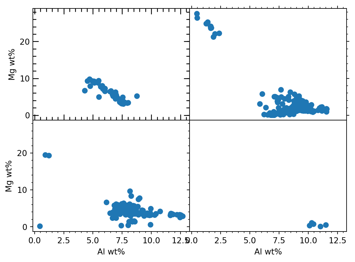
Practise: Selecting a Plot- Prodcue a figure with 4 individual plots that share the y-axis. Define a variable ‘sel’, and depending on its value make the plots with space between all of them, or no sapace between the plots in the columns.
import matplotlib.pyplot as plt

space = True

if space == True:
    wsWidth = .1
else:
    wsWidth = 0

fig, ((ax1, ax2), (ax3, ax4)) = plt.subplots(2, 2, sharey = True)
fig.subplots_adjust(hspace = 0, wspace = wsWidth)

ax1.scatter([1,2,3], [4,5,6])
ax2.scatter([7,8,9], [1,2,3])
ax3.scatter([4,5,6], [7,8,9])
ax4.scatter([3,2,1], [4,5,6])

plt.show()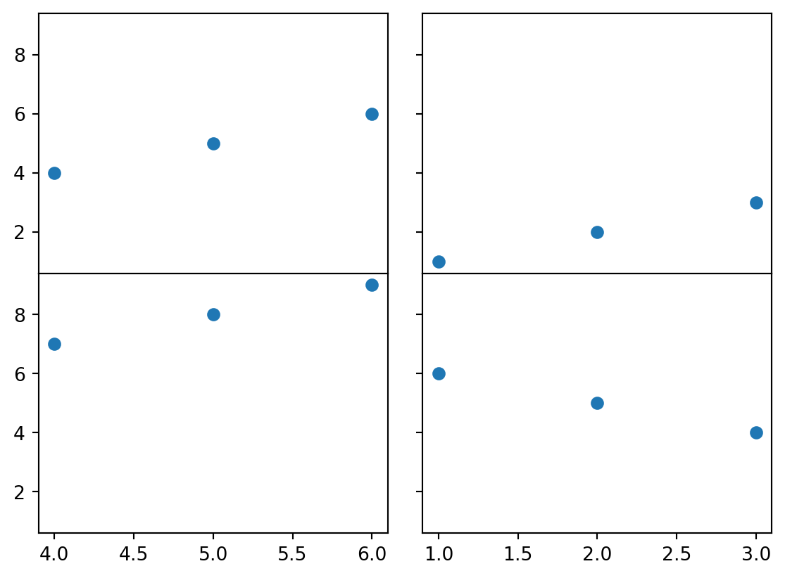
5.3 Basics - list comprehension [05:01]
list comprehension
Häufig verwenden wir eine Schleife, um eine Operation auf die einzelnen Elemente einer Liste anzuwenden, und das Ergebni in eine neue Schleife zu schreiben. Für den Fall einer kurzen Schleife gibt es eine Kurzschreibweise, welche den Code knackig verkürzt.
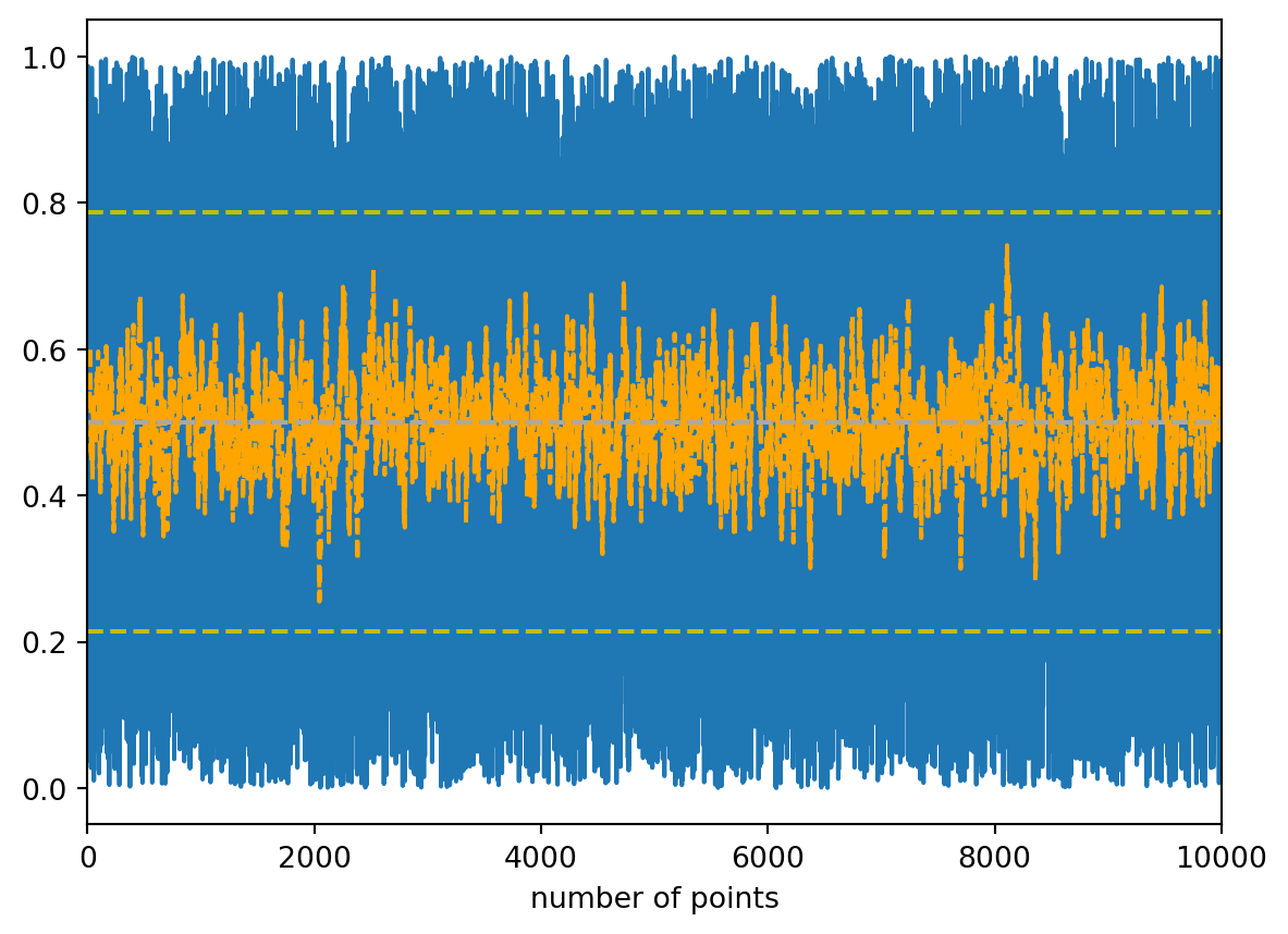
5.4 Statistics - mean, median, stdev, moving average [22:38]
mean, median, standard deviation, moving average, list comprehension
Zum Einstieg in statistische Methoden gibt es einen ersten Blick auf Mittelwert, Median, Standardabweichung und gleitenden Durchschnitt (moving average).
Video nb
import numpy as np
import matplotlib.pyplot as plt
max_points = 10000
batch_size = 20
random_numbers = np.random.rand(max_points)
calc_mean = np.mean(random_numbers)
calc_median = np.median(random_numbers)
calc_std = np.std(random_numbers)
moving_mean = [np.mean(random_numbers[i - batch_size:i]) for i in range(len(random_numbers))]
plt.plot(random_numbers)
plt.plot(moving_mean, c='orange', linestyle='dashed')
plt.axhline(calc_mean, c='grey', linestyle='dashed')
plt.axhline(calc_median, c='darkgrey', linestyle='dashed')
plt.axhline(calc_mean - calc_std, c='y', linestyle='dashed')
plt.axhline(calc_mean + calc_std, c='y', linestyle='dashed')
plt.xlabel('number of points')
plt.xlim([0,max_points])
plt.show()/Users/dominik/anaconda3/lib/python3.11/site-packages/numpy/core/fromnumeric.py:3504: RuntimeWarning:
Mean of empty slice.
/Users/dominik/anaconda3/lib/python3.11/site-packages/numpy/core/_methods.py:129: RuntimeWarning:
invalid value encountered in scalar divide
Practise: Instead of a moving average, plot the moving median of a list with random numbers.
Simply replace np.mean with np.median - and rename the respectvive variables accordingly.
import numpy as np
import matplotlib.pyplot as plt
max_points = 10000
batch_size = 20
random_numbers = np.random.rand(max_points)
calc_mean = np.mean(random_numbers)
calc_median = np.median(random_numbers)
calc_std = np.std(random_numbers)
moving_median = [np.median(random_numbers[i - batch_size:i]) for i in range(len(random_numbers))]
plt.plot(random_numbers)
plt.plot(moving_median, c='orange', linestyle='dashed')
plt.axhline(calc_mean, c='grey', linestyle='dashed')
plt.axhline(calc_median, c='darkgrey', linestyle='dashed')
plt.xlabel('number of points')
plt.xlim([0,max_points])
plt.show()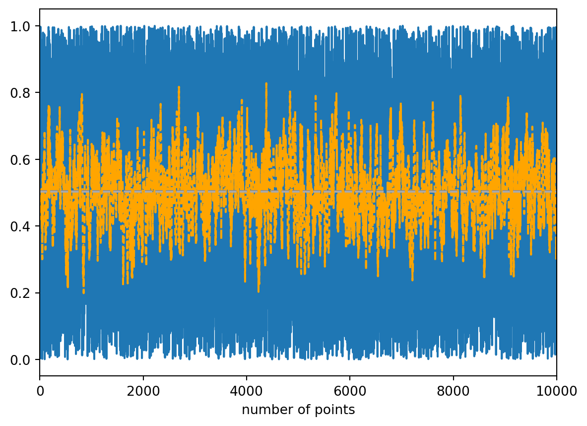
5.5 Statistics - example of a moving average [07:18]
moving average, stocks
Als ein bekanntes Beispiel mit einfachem online-Zugriff schauen wir uns den moving average von Aktien-Preisen an.
Video nb
import yfinance as yf
import pandas as pd
import matplotlib.pyplot as plt
from datetime import datetime

batch_days = 365
today = datetime.today().strftime('%Y-%m-%d')

ticker = 'AAPL'
stock_data = yf.download(ticker, start='2020-01-01', end=today)

plot_data = [stock_data['Close'][i-batch_days:i].mean() for i in range(len(stock_data['Close']))]

plt.plot(stock_data.index, stock_data['Close'])
plt.plot(stock_data.index, plot_data)
plt.show()
YF.download() has changed argument auto_adjust default to True[*********************100%***********************] 1 of 1 completed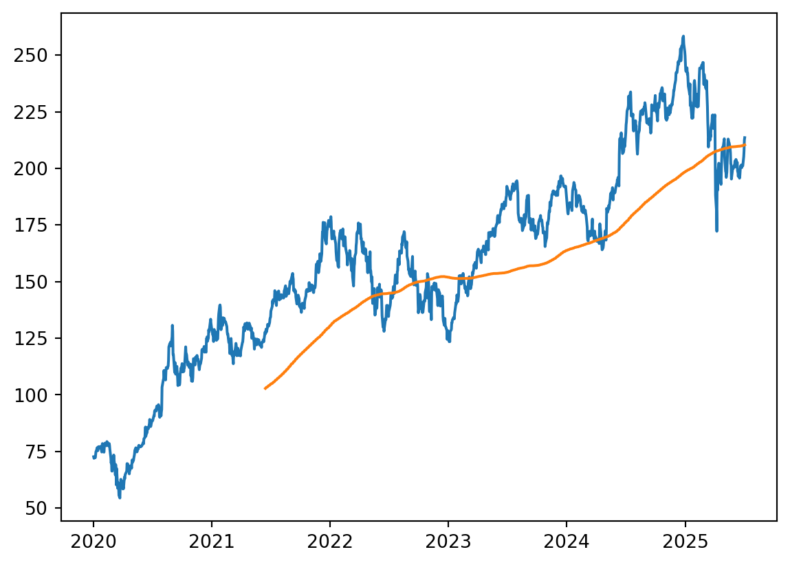
Practise: Produce a plot including the moving average of global, historic temperature data. (Additional practise info is provided at the start of this callout.)
Copy the content of the first 2 cells to your notebook, run them, and start with the df defined at the end of these to solve this practise. This df contains a ready to use global, historic temperature dataset.
The solution video further below explains the entire code in detail.
import pandas as pd
import matplotlib.pyplot as plt
from ipywidgets import interact
Donwloading and plotting the temperature data only.
url = "https://berkeley-earth-temperature.s3.us-west-1.amazonaws.com/Global/Complete_TAVG_complete.txt"

df = pd.read_csv(url, comment="%", sep='\s+'
    ,names=['Year', 'Month',  'Anomaly']
    ,usecols=[0, 1, 2])

df["date"] = pd.to_datetime(dict(year=df['Year'], month=df['Month'], day=15))

df = df[['date', 'Anomaly']]
df.head()| date | Anomaly | |
|---|---|---|
| 0 | 1750-01-15 | -0.252 |
| 1 | 1750-02-15 | -1.261 |
| 2 | 1750-03-15 | 0.225 |
| 3 | 1750-04-15 | 0.288 |
| 4 | 1750-05-15 | -0.970 |
plt.plot(df['date'], df['Anomaly'])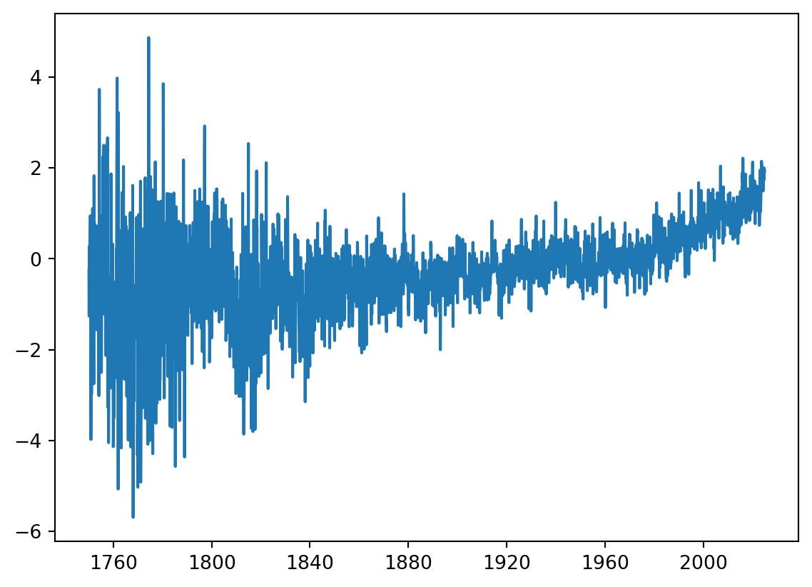
Adding the moving temperature average.
The slider is not evaluated in this online book, i.e., there is no change on the plot when sliding the slider up or down.
def global_T_mov_av(batch_size):
    data = df['Anomaly']
    data2 = [np.mean(data[i-batch_size:i]) for i in range(batch_size, len(data))]

    plt.plot(df['date'], data)
    plt.plot(df['date'][batch_size:], data2)
    plt.xlabel('time')
    plt.ylabel('global temperature anomaly (ºC)')
    return plt.show()

interact(global_T_mov_av, batch_size = (1, 100, 1))
<function __main__.global_T_mov_av(batch_size)>Storing the downloaded and manipulated data locally in your file system und the specified path, if desired.
df.to_csv(your_path + 'historic global temperature anomalies.txt', index=False)