pip install mag4Requirement already satisfied: mag4 in /Users/dominik/anaconda3/lib/python3.11/site-packages (0.0.214)
Note: you may need to restart the kernel to use updated packages.In den vergangenen Jahren werden immer mehr Daten publiziert, deren Menge zukünftig noch schneller anwachsen wird. Es ist nicht leicht, all den Publikationen dieser erfreulich großen Mengen immer neuer Informationen zu folgen. Jupyter Notebooks wurden gerade auch dafür entwickelt, auf große Mengen an Daten zuzugreifen, diese zu visualisieren, analysieren und auf Problemstellungen anzuwenden. Natürlich ist das nur möglich, wenn die Daten in entsprechenden Formaten vorliegen. Oftmals ist daher im ersten Schritt ein ›Daten clean-up‹ notwendig. Seit 2020 gibt es nun endlich mehrere Initiativen, darunter so große wie die Nationale Forschungsdatenbank Initiative (NFDI) der DFG, GWK und anderer, die versuchen gemeinsam mit internationalen Partnern Daten besser verfügbar zu machen. Schon bestehende Datenbanken wie GeoROC, EarthChem oder auch MetBase erlauben schon seit langer Zeit solchen Zugang, und damit Data Science in z.B. der Geo- und Kosmochemie. In dieser Einheit steigen wir in das neue Feld der Data Science in der Mineralogie ein.
Zunächst müssen wir uns etwas anschauen, wie Datensätze und eine Datenbank überhaupt aufgebaut sind. Wir sind zwar sehr damit vertraut, Tabellen zu erstellen, als Datenbank taugen die meisten jedoch selten etwas. Datenbanken, bzw. einzelne Datensätze erstellt man mit einigen wenigen, einfachen Regeln, die wir nun kennen lernen wollen – danach sehen auch die meisten Tabellen besser aus. Außerdem lernen wir noch ein wenig hilfreiches, und Datenbank bezogenen Vokabular kennen.
pandas: shape(), info, columns, set_option(›display.max_rows’, 20), python: type() set_option(‘display.max_rows’, 20), drop_duplicates(), df[›category name‹], >, <, &
Available Notebooks: Lecture, Exercise, Solution
Python selbst stellt nur einen sehr begrenzten Umfang an Befehlen zur Daten-Manipulation zur verfügung. Allerdings gibt es sehr viele zusätzliche Befehlspakete – genannt: libraries oder packages – für alles mögliche, auch eines zur Daten-Manipulation. Diese heißt (warum auch immer) ›pandas‹, und dessen Grundzüge lernen wir nun kennen.
read_csv(), maptplotlib.pyplot, plt, plot(), scatter(), show(), xlabel(), legend(), xlim()
Available Notebooks: Lecture, Exercise, Solution
Eine weitere library ist die ›matplotlib‹, die praktische alle nur denkbaren Plots und deren noch so komplizierten Darstellungen ermöglicht. In diese nehmen wir nun einen ersten, kleinen Einblick.
import mag4 as mg
import pandas as pd
import matplotlib.pyplot as pltdf_minData = mg.get_data('Mineral Data Example Dataset')
df_mydata = mg.get_data('Mineral Data Example Dataset 2')A simple line plot
el = 'MnO'
plt.plot(df_minData[el])
plt.show()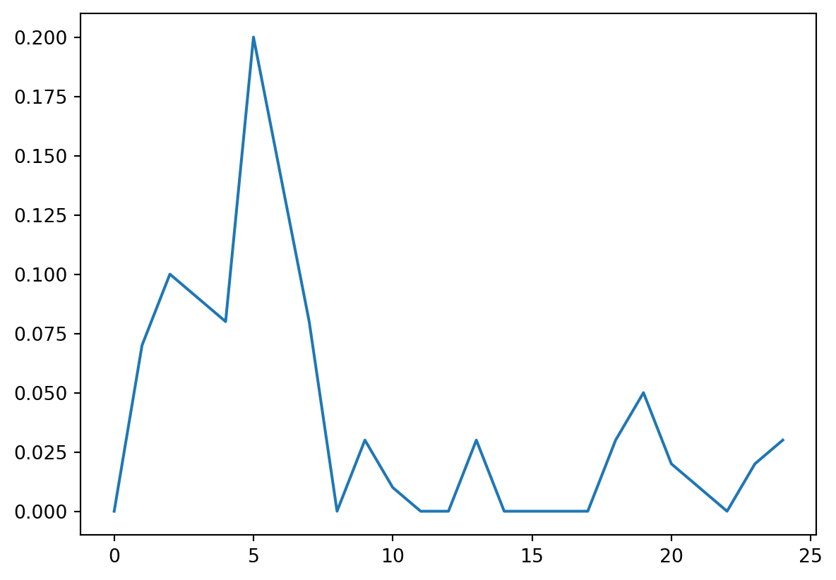
A simple scatter plot
el1 = 'MgO'
el2 = 'SiO2'
plt.scatter(df_minData[el1], df_minData[el2])
plt.show()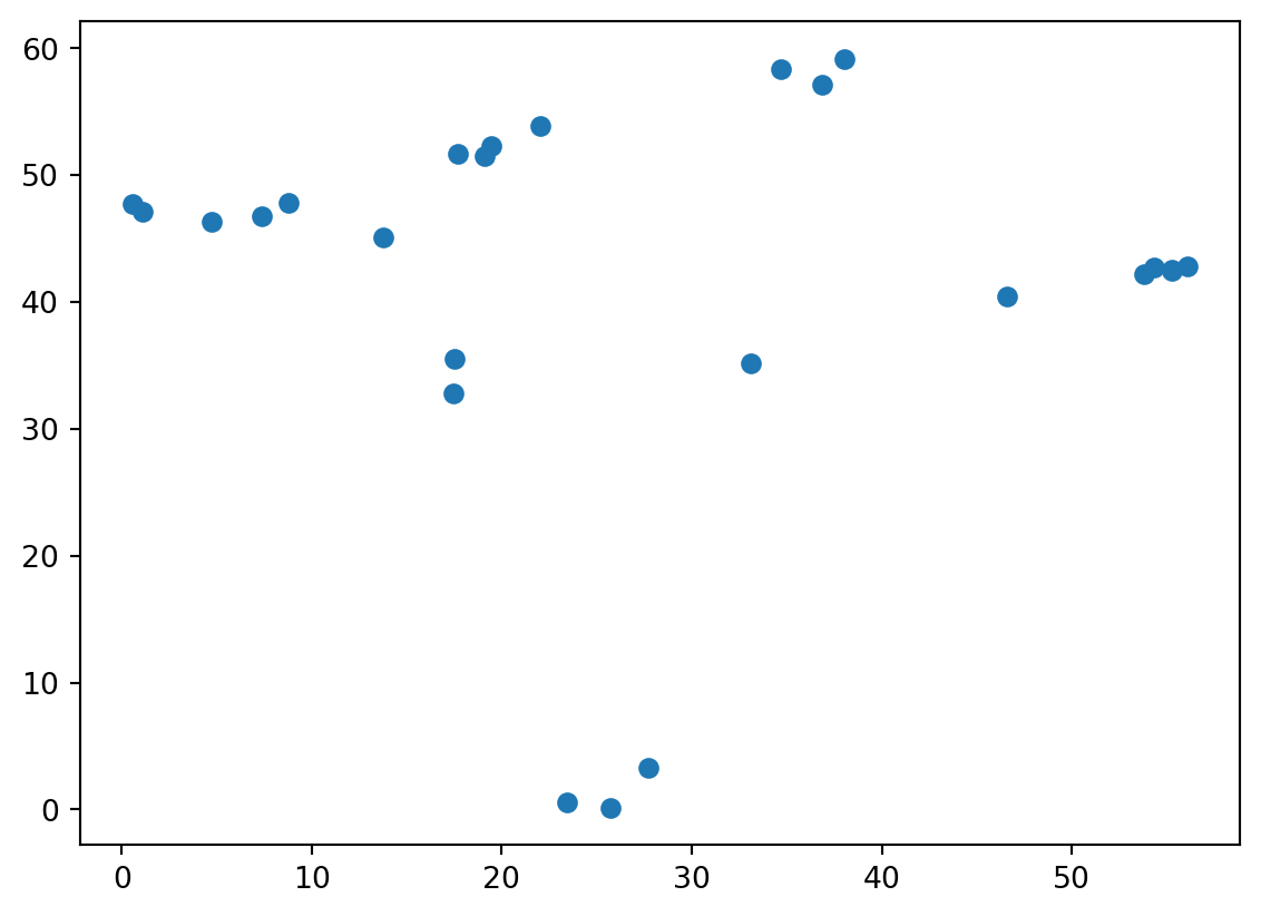
Formating elements
el1 = 'MnO'
el2 = 'SiO2'
plt.scatter(df_minData[el1], df_minData[el2], label = 'Mineral Example Data')
plt.scatter(df_mydata[el1], df_mydata[el2], label = 'Mineral Example Data 2')
plt.xlabel(el1)
plt.ylabel(el2)
plt.legend(loc = 'lower right')
plt.xlim(0, 0.22)
plt.ylim(0, 60)
plt.show()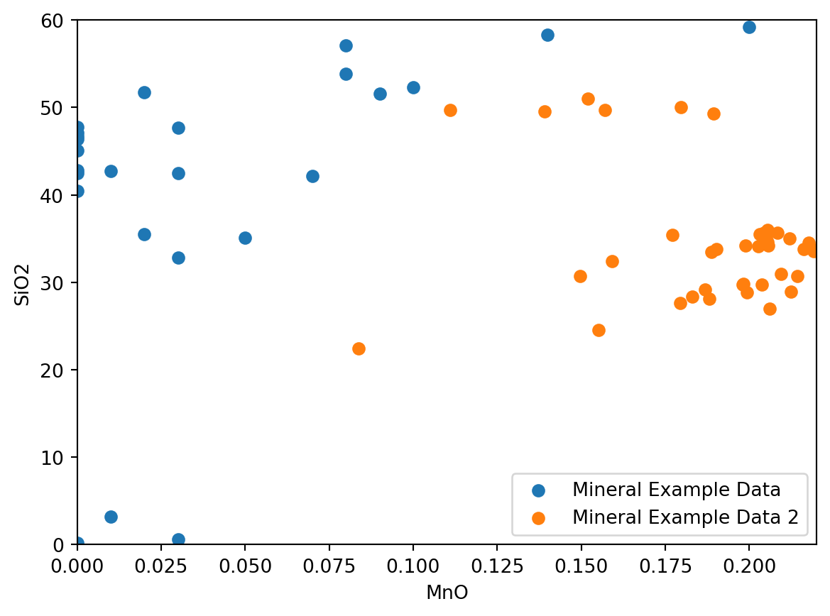
Start with importing the pandas and matplotlib libraries.
Then read the example file Mineral Data Example Dataset 3, and store it a variable.
Display the categories and the data table. Use .tolist() to display the categories in a compact form.
Then plot the FeO data on the y-axis and label it with FeO.
Make the code flexibel, so that FeO can be quickly replaced by another oxide.
Then plot two oxides against each other, again flexible, and add a legend.
Finally, add data from the file Mineral Data Example Dataset to the latter plot.
import mag4 as mg
import pandas as pd
import matplotlib.pyplot as pltdf = mg.get_data('Mineral Data Example Dataset 3')
print(df.columns.tolist())
df['No.', 'SiO2', 'TiO2', 'Al2O3', 'FeO', 'MnO', 'MgO', 'CaO', 'Na2O', 'K2O', 'P2O5', 'Cr2O3', 'NiO', 'Total', 'Comment']| No. | SiO2 | TiO2 | Al2O3 | FeO | MnO | MgO | CaO | Na2O | K2O | P2O5 | Cr2O3 | NiO | Total | Comment | |
|---|---|---|---|---|---|---|---|---|---|---|---|---|---|---|---|
| 0 | 1 | 57.2700 | 1.6275 | 17.9100 | 6.4200 | 0.1614 | 2.2800 | 3.46 | 4.4600 | 5.4500 | 0.8939 | 0.0026 | 0.0000 | 99.9354 | GProbe Mitte Grid 010x011 Grid 020x021 |
| 1 | 2 | 57.2800 | 1.5939 | 18.0100 | 6.4400 | 0.1372 | 2.3100 | 3.49 | 4.4300 | 5.4300 | 0.8622 | 0.0000 | 0.0070 | 99.9903 | GProbe Mitte Grid 010x011 Grid 020x021 |
| 2 | 4 | 57.1600 | 1.6335 | 18.0300 | 6.4500 | 0.1535 | 2.3000 | 3.48 | 4.4700 | 5.4300 | 0.9481 | 0.0109 | 0.0163 | 100.0823 | GProbe Mitte Grid 010x011 Grid 020x021 |
| 3 | 5 | 57.3100 | 1.6235 | 17.9800 | 6.4300 | 0.1502 | 2.2700 | 3.48 | 4.3800 | 5.4300 | 0.9043 | 0.0000 | 0.0000 | 99.9580 | GProbe Mitte Grid 010x011 Grid 020x021 |
| 4 | 7 | 57.3900 | 1.6314 | 18.0800 | 6.5100 | 0.1466 | 2.2900 | 3.51 | 4.4000 | 5.4400 | 0.8663 | 0.0161 | 0.0000 | 100.2804 | GProbe Mitte Grid 010x011 Grid 020x021 |
| ... | ... | ... | ... | ... | ... | ... | ... | ... | ... | ... | ... | ... | ... | ... | ... |
| 192 | 287 | 1.3845 | 0.0000 | 0.0045 | 0.0010 | 0.0000 | 1.3767 | 49.92 | 0.0713 | 0.0000 | 0.0104 | 0.0070 | 0.0000 | 52.7754 | GProbe Mitte Grid 010x011 Grid 020x021 |
| 193 | 289 | 0.7298 | 0.0082 | 0.0000 | 0.0333 | 0.0000 | 1.4190 | 49.99 | 0.0640 | 0.0000 | 0.0128 | 0.0000 | 0.0000 | 52.2571 | GProbe Mitte Grid 010x011 Grid 020x021 |
| 194 | 290 | 0.6210 | 0.0072 | 0.0006 | 0.0060 | 0.0000 | 1.3827 | 50.26 | 0.0655 | 0.0000 | 0.0000 | 0.0046 | 0.0000 | 52.3476 | GProbe Mitte Grid 010x011 Grid 020x021 |
| 195 | 292 | 0.5870 | 0.0000 | 0.0000 | 0.0072 | 0.0000 | 1.3888 | 50.19 | 0.0542 | 0.0026 | 0.0000 | 0.0000 | 0.0000 | 52.2299 | GProbe Mitte Grid 010x011 Grid 020x021 |
| 196 | 293 | 0.6773 | 0.0000 | 0.0084 | 0.0000 | 0.0000 | 1.4192 | 50.44 | 0.0713 | 0.0000 | 0.0002 | 0.0216 | 0.0143 | 52.6523 | GProbe Mitte Grid 010x011 Grid 020x021 |
197 rows × 15 columns
el = 'FeO'
plt.plot(df[el])
plt.ylabel(el)
plt.show()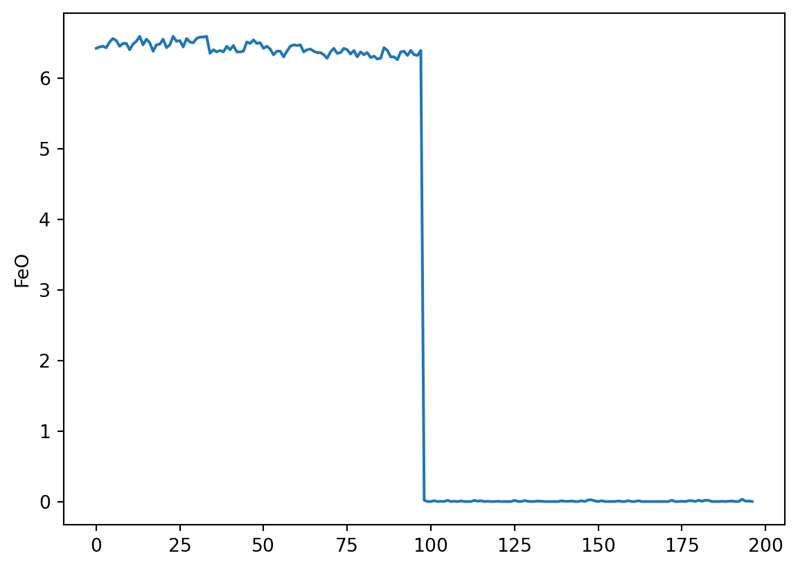
el1 = 'MnO'
el2 = 'FeO'
plt.scatter(df[el1], df[el2], label = 'Mineral Example Dataset 3')
plt.xlabel(el1)
plt.ylabel(el2)
plt.legend(loc = 'lower right')
plt.show()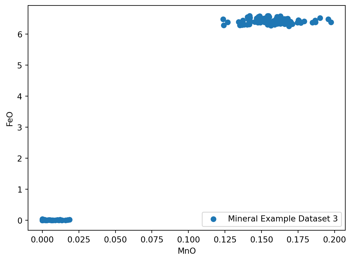
df_minData = mg.get_data('Mineral Data Example Dataset')el1 = 'MnO'
el2 = 'FeO'
plt.scatter(df[el1], df[el2], label = 'Mineral Example Dataset 3')
plt.scatter(df_minData[el1], df_minData[el2], label = 'Mineral Data')
plt.xlabel(el1)
plt.ylabel(el2)
plt.legend(loc = 'upper left')
plt.show()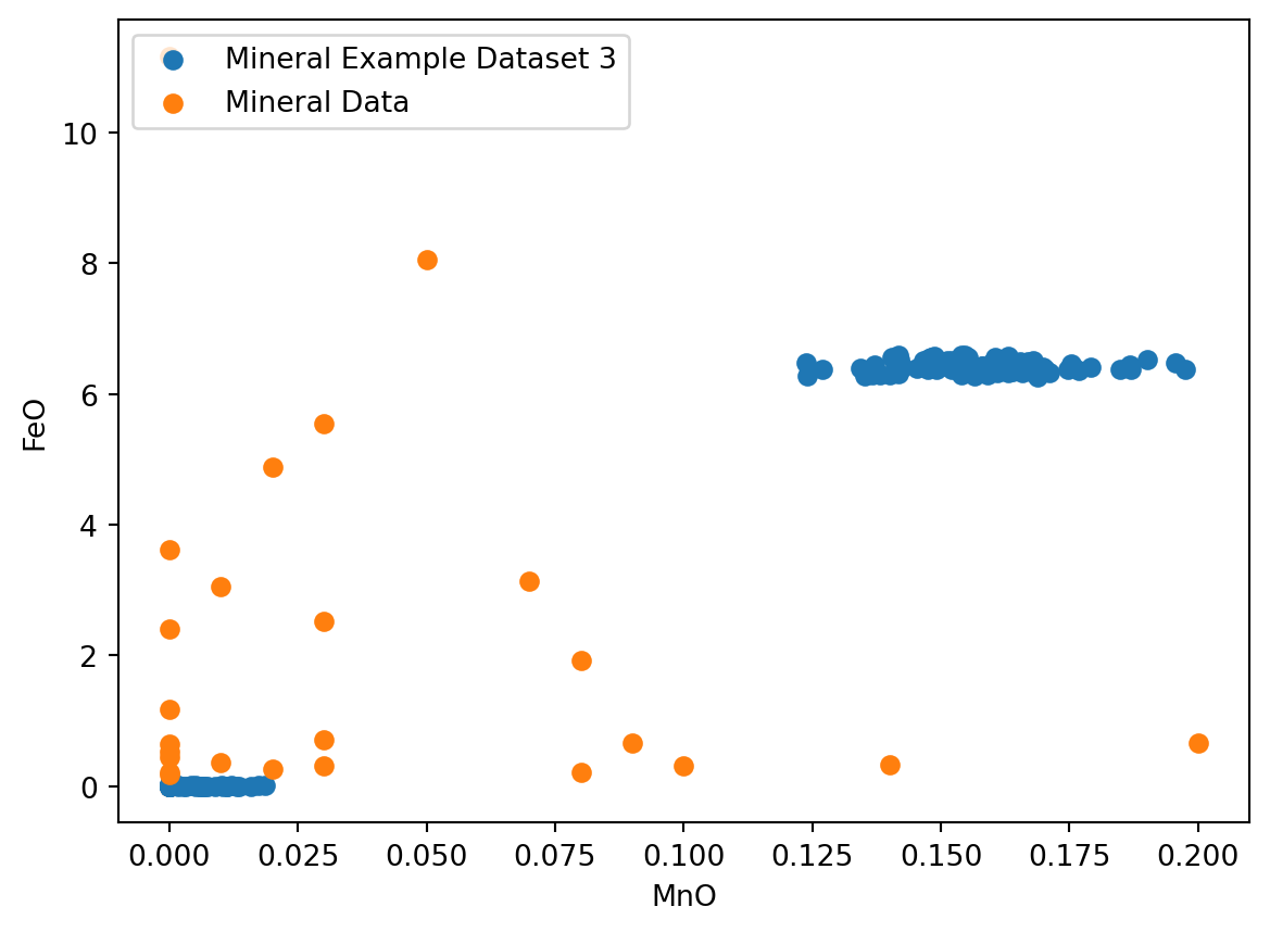
.iloc(), .loc(), .set_index()
Available Notebooks: Lecture, Exercise, Solution
Nun wollen wir lernen, wie leicht mit Pandas jegliche gewünschten Daten aus einer Datenbank, also z.B. einer einfachen Excel-Tabelle extrahiert werden können. Das ist besonders wichtig und hilfreich, wenn die Datenbank sehr groß ist, oder wenn man immer andere Datenbanken verwendet, die aber immer anders aufgebaut sind. Anders aufgebaut meint, dass z.B. die Kategorienamen in anderer Reihenfolge stehen, oder evtl. auch etwas anders lauten. Dann müsste bei einem Code mit Pandas nur der entsprechende Kategoriename geändert werden, der Code selbst bliebe gleich.
Available Notebooks: Lecture, Exercise, Solution
Zum Schluss dieser Einheit wollen wir die geballte Kraft von Pandas mit der von maplotlib kombinieren. D.h., wir selektieren zunächst mit Pandas die gewünschten Daten aus einer Datenbank, und visualisieren diese umgehend und einfach mit Hilfe der matplotlib Bibliothek.
import mag4 as mg
import pandas as pd
import matplotlib.pyplot as pltdf = mg.get_data('Banda Arc')
data = df.loc[3:9, ['Mg', 'Si', 'Mn']]
el1 = 'Mg'
plt.scatter(data[el1], data['Mn'])
plt.xlabel(el1)Text(0.5, 0, 'Mg')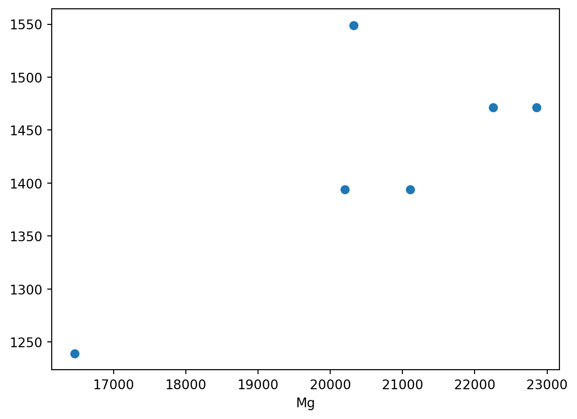
Import the 2 databases we require for plotting, plus the one to load data.
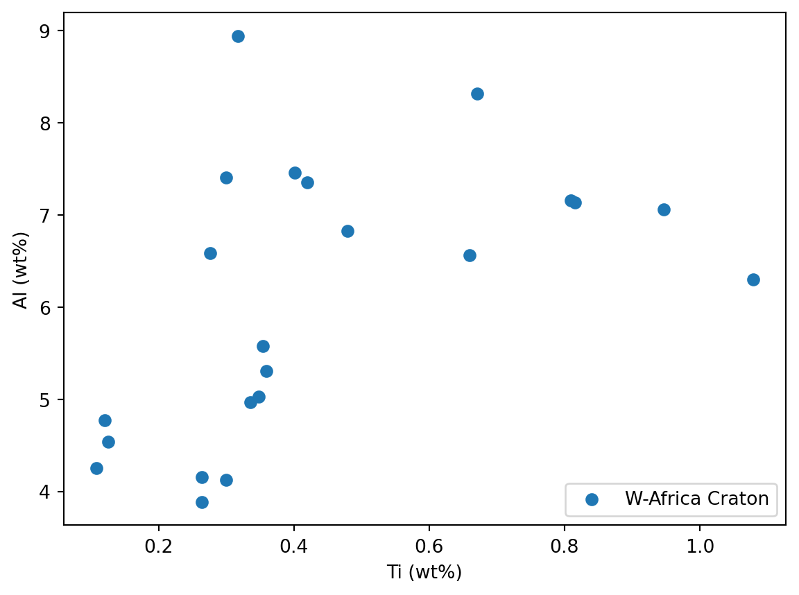
Then, we need a database, which shall be West African Craton, and as usual we want to display some sensible information.
Then display datasets 5 through 25, and flexibly plot two elements against each other that are also shown as lables on the respective axes, as well as a legend indicating what data are shown.
The data are in wt-ppm. Change this to wt%.
If we want to concatenate strings, we can simply do this using + between two strings, e.g.: 'a' + 'b', which will result in 'ab'. Try using this to add units to the axes labelling.
import mag4 as mg
import pandas as pd
import matplotlib.pyplot as plt
df = mg.get_data('West African Craton')
print(df.columns.tolist())
df['Citations', 'Tectonic Setting', 'Location', 'Location Comment', 'Latitude (Min)', 'Latitude (Max)', 'Longitude (Min)', 'Longitude (Max)', 'Land or Sea', 'Elevation (Min)', 'Elevation (Max)', 'Sample Name', 'Rock Name', 'Age (a, Min)', 'Age (a, Max)', 'Geol', 'Age', 'Eruption Day', 'Eruption Month', 'Eruption Year', 'Rock Texture', 'Rock Type', 'Drill Depth (Min)', 'Drill Depth (Max)', 'Alteration', 'Mineral', 'Material', 'Si', 'Ti', 'B', 'Al', 'Cr', 'Fe3+', 'Fe2+', 'Fetot(2+)', 'Ca', 'Mg', 'Mn', 'Ni', 'K', 'Na', 'P', 'H2O', 'H2OP', 'H2OM', 'H2Otot', 'CO2', 'CO', 'F', 'Cl', 'Cl2', 'OH', 'CH4', 'SO2', 'SO3', 'SO4', 'S', 'LOI', 'Volatiles', 'O', 'Others', 'HE(CCM/G)', 'HE(CCMSTP/G)', 'HE3(CCMSTP/G)', 'HE3(AT/G)', 'HE4(CCM/G)', 'HE4(CCMSTP/G)', 'HE4(AT/G)', 'HE4(MOLE/G)', 'HE4(NCC/G)', 'HE(NCC/G)', 'Li', 'Be', 'B.1', 'C', 'CO2.1', 'F.1', 'Na.1', 'Al.1', 'P.1', 'S.1', 'Cl.1', 'K.1', 'Ca.1', 'Sc', 'Ti.1', 'V', 'Cr.1', 'Mn.1', 'Fe', 'Co', 'Ni.1', 'Cu', 'Zn', 'Ga', 'Ge', 'As', 'Se', 'Br', 'Rb', 'Sr', 'Y', 'Zr', 'Nb', 'Mo', 'Ru', 'Rh', 'Pd', 'Ag', 'Cd', 'In', 'Sn', 'Sb', 'Te', 'I', 'Cs', 'Ba', 'La', 'Ce', 'Pr', 'Nd', 'Sm', 'Eu', 'Gd', 'Tb', 'Dy', 'Ho', 'Er', 'Tm', 'Yb', 'Lu', 'Hf', 'Ta', 'W', 'Re', 'Os', 'Ir', 'Pt', 'Au', 'Hg', 'Tl', 'Pb', 'Bi', 'Th', 'U', 'Nd143/Nd144', 'Nd143/Nd144 initial', 'e Nd', 'Sr87/Sr86', 'SR87_SR86_INI', 'PB206_PB204', 'PB206_PB204_INI', 'PB207_PB204', 'PB207_PB204_INI', 'PB208_PB204', 'PB208_PB204_INI', 'OS184_OS188', 'OS186_OS188', 'OS187_OS186', 'OS187_OS188', 'RE187_OS186', 'RE187_OS188', 'HF176_HF177', 'HE3_HE4', 'HE3_HE4(R/R(A))', 'HE4_HE3', 'HE4_HE3(R/R(A))', 'K40_AR40', 'AR40_K40', 'Unique Id']| Citations | Tectonic Setting | ... | AR40_K40 | Unique Id | |
|---|---|---|---|---|---|
| 0 | [5205] | ARCHEAN CRATON (INCLUDING GREENSTONE BELTS) | ... | NaN | 184947 |
| 1 | [5205] | ARCHEAN CRATON (INCLUDING GREENSTONE BELTS) | ... | NaN | 184948 |
| ... | ... | ... | ... | ... | ... |
| 41 | [8624] | ARCHEAN CRATON (INCLUDING GREENSTONE BELTS) | ... | NaN | 247031 |
| 42 | [8624] | ARCHEAN CRATON (INCLUDING GREENSTONE BELTS) | ... | NaN | 247032 |
43 rows × 170 columns
el1 = 'Ti'
el2 = 'Al'

xData = df.loc[5:26, el1]
yData = df.loc[5:26, el2]

plt.scatter(xData, yData, label = 'W-Africa Craton')
plt.xlabel(el1)
plt.ylabel(el2)
plt.legend(loc = 'lower right')

plt.show()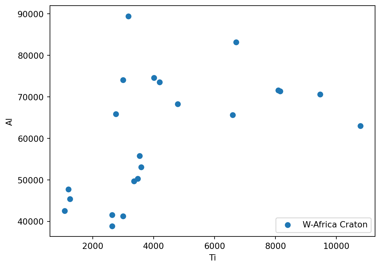
el1 = 'Ti'
el2 = 'Al'

xData = df.loc[5:26, el1] / 10000
yData = df.loc[5:26, el2] / 10000

plt.scatter(xData, yData, label = 'W-Africa Craton')
plt.xlabel(el1 + ' (wt%)')
plt.ylabel(el2 + ' (wt%)')
plt.legend(loc = 'lower right')

plt.show()