4 Interaktive Elemente & erste Programme [41:42]

Nun fehlt uns nur noch wenig Rüstzeug, um erste, leistungsfähige Programme zu schreiben. Dieses Verbleibende lernen wir in dieser Einheit, um dann tatsächlich 2 Programme zu bauen, welche Datenbank-Daten effektiv darstellen. Vor allem lernen wir hier interaktive Möglichkeiten kennen die es uns ermöglichen, mit den Daten über eine graphische Benutzeroberfläche direkt zu interagieren, diese zu manipulieren und immer wieder neu darzustellen.

4.1 Basics- local & global variables [05:05]

global
Available Notebooks: Lecture, Exercise, Solution

Lokale Variablen gelten nur innerhalb bestimmter Befehle. Das ist sehr praktisch, da derselbe Variablen-Name ohne Konflikte dann noch woanders verwendet werden kann. Globale Variablen gelten dagegen überall, sodass eine Doppelbelegung unbedingt vermieden werden muss.

Video nb

a = 4
a

Global variable

test = 14

for test in [1, 2, 3, 4]:
    print(test + 3)
    
test

Local variable

res = 6

def addOne(n):
    #global res   # this line would make res a global variable
    res = n + 1   # res is a local variable within def
    return res

addOne(4)

res

Give an example for a local variable and its behaviour.

Variables within self-defined commands (def) are local varibales. These variables have either no value outside this self-defined command, or any other value, that has been assigend to this variable outside the command.
The value of global variables is valid anywhere in a code – except for where these are local variables, e.g., wihtin self-defined commands.

The value in a for loop – e.g., the ‘n’ in for n in … is a always a local variable.

✗True

False

Variables within self-defined commands can be made global.

True

✗False

Practise

We have the following list with Mg concentrations:

mg = [22.13, 18.45, 19.26, 21.76]  # in wt%

The conversion factor from Mg element to oxide wt% is 1.658.
Write a command called ‘convertMgToMgO’ that converts the entire mg list into an mgo list.
Use a local varibale for the conversion factor from mg to mgo.
Execute the command to test it. Make sure, only 2 decimals are shown.
Check that your variable really is local by executing it.

Solution

def convertMgToMgO(l):
    conv = 1.658
    res = []
    for n in l:
        res.append(round(conv * n, 2))
    return res

convertMgToMgO(mg)

[36.69, 30.59, 31.93, 36.08]

What’s wrong with this code? (NONE YET)

coming

Solution

coming

4.2 Basics- Introduction to interactive elements [09:24]

ipywidgets library, interact(), concatenate strings (+)
Available Notebooks: Lecture, Exercise, Solution

Interaktive Elemente erlauben es Anwendern die dargestellten Inhalte – also beispielsweise ein Diagramm – zu manipulieren, also damit zu interagieren. So können über Drop-Down Menüs z.B. die darzustellenden chemischen Elemente ausgewählt, oder über Slider Variablen-Werte verändert werden. Diese Elemente bilden eine GUI (graphical user interface), mit der sich richtige Programme erstellen lassen.

Video nb

pip install mag4

Requirement already satisfied: mag4 in /Users/dominik/anaconda3/lib/python3.11/site-packages (0.0.214)
Note: you may need to restart the kernel to use updated packages.

import mag4 as mg
import pandas as pd
import matplotlib.pyplot as plt
from ipywidgets import interact

df = mg.get_data('Bastar Craton')
print(df.columns.tolist())

['Citations', 'Tectonic Setting', 'Location', 'Location Comment', 'Latitude (Min)', 'Latitude (Max)', 'Longitude (Min)', 'Longitude (Max)', 'Land or Sea', 'Elevation (Min)', 'Elevation (Max)', 'Sample Name', 'Rock Name', 'Age (a, Min)', 'Age (a, Max)', 'Geol', 'Age', 'Eruption Day', 'Eruption Month', 'Eruption Year', 'Rock Texture', 'Rock Type', 'Drill Depth (Min)', 'Drill Depth (Max)', 'Alteration', 'Mineral', 'Material', 'Si', 'Ti', 'B', 'Al', 'Cr', 'Fe3+', 'Fe2+', 'Fetot(2+)', 'Ca', 'Mg', 'Mn', 'Ni', 'K', 'Na', 'P', 'H2O', 'H2OP', 'H2OM', 'H2Otot', 'CO2', 'CO', 'F', 'Cl', 'Cl2', 'OH', 'CH4', 'SO2', 'SO3', 'SO4', 'S', 'LOI', 'Volatiles', 'O', 'Others', 'HE(CCM/G)', 'HE(CCMSTP/G)', 'HE3(CCMSTP/G)', 'HE3(AT/G)', 'HE4(CCM/G)', 'HE4(CCMSTP/G)', 'HE4(AT/G)', 'HE4(MOLE/G)', 'HE4(NCC/G)', 'HE(NCC/G)', 'Li', 'Be', 'B.1', 'C', 'CO2.1', 'F.1', 'Na.1', 'Mg.1', 'Al.1', 'P.1', 'S.1', 'Cl.1', 'K.1', 'Ca.1', 'Sc', 'Ti.1', 'V', 'Cr.1', 'Mn.1', 'Fe', 'Co', 'Ni.1', 'Cu', 'Zn', 'Ga', 'Ge', 'As', 'Se', 'Br', 'Rb', 'Sr', 'Y', 'Zr', 'Nb', 'Mo', 'Ru', 'Rh', 'Pd', 'Ag', 'Cd', 'In', 'Sn', 'Sb', 'Te', 'I', 'Cs', 'Ba', 'La', 'Ce', 'Pr', 'Nd', 'Sm', 'Eu', 'Gd', 'Tb', 'Dy', 'Ho', 'Er', 'Tm', 'Yb', 'Lu', 'Hf', 'Ta', 'W', 'Re', 'Os', 'Ir', 'Pt', 'Au', 'Hg', 'Tl', 'Pb', 'Bi', 'Th', 'U', 'Nd143/Nd144', 'Nd143/Nd144 initial', 'e Nd', 'Sr87/Sr86', 'SR87_SR86_INI', 'PB206_PB204', 'PB206_PB204_INI', 'PB207_PB204', 'PB207_PB204_INI', 'PB208_PB204', 'PB208_PB204_INI', 'OS184_OS188', 'OS186_OS188', 'OS187_OS186', 'OS187_OS188', 'RE187_OS186', 'RE187_OS188', 'HF176_HF177', 'HE3_HE4', 'HE3_HE4(R/R(A))', 'HE4_HE3', 'HE4_HE3(R/R(A))', 'K40_AR40', 'AR40_K40', 'Unique Id', 'Unnamed: 171']

el1 = 'Na'
el2 = 'Mn'

plt.scatter(df[el1], df[el2])

plt.show()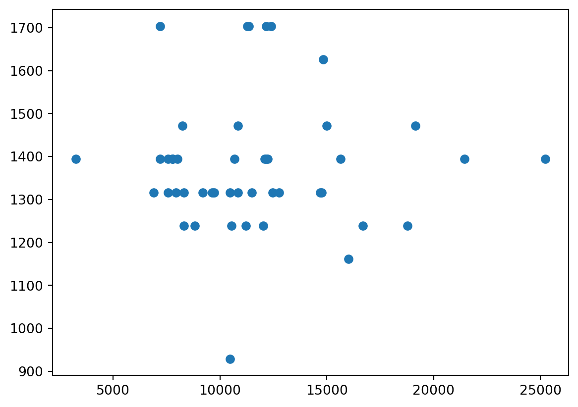

def pltData(xAxisData, yAxisData):
    plt.scatter(df[xAxisData] / 10000, df[yAxisData] / 10000)
    plt.xlabel(xAxisData + ' (wt%)')
    plt.ylabel(yAxisData + ' (wt%)')
    return plt.show()

el1 = 'Mn'
el2 = 'Ti'

pltData(el1, el2)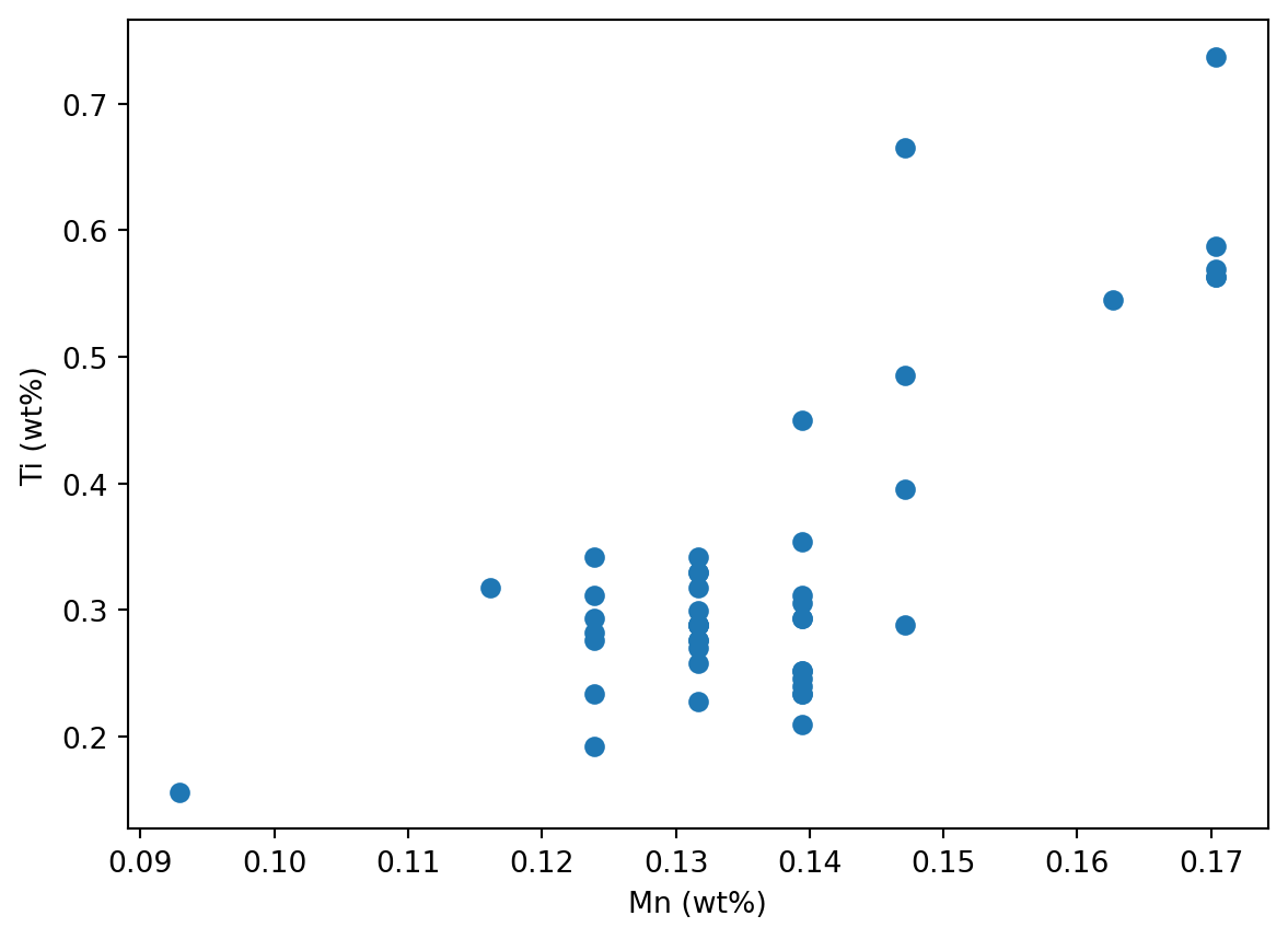

elements = ['Si', 'Ti', 'Al', 'Mg', 'Mn', 'V']

interact(pltData, xAxisData = elements, yAxisData = elements)

<function __main__.pltData(xAxisData, yAxisData)>

What are interactive elements?

Baiscally GUI (graphical user interface) elements, with which a user can interact with the displayed or visualised data.

What is required for interactive elements?

✗A self-defined method

✗A self-defined for loop

✓A self-defined command

✗Nothing particular

Interact can take a maximum of 5 variables.

✗True

✓False

Practise

Import the required libraries to make an interactive plot using a database.
As database we want to use ‘Tanzania Craton Archean’.
Make a scatter plot including some labelling elements.
Now make a command that makes this plot, with the two elements as input variables to the command.
Execute the command to test it.
Now use interact to select the elements for the x- and y-axes via drop-down menus.
Use a list with elements that will populate the drop-down menus.
Finally, test and enjoy that all is working just fine.

Solution

import mag4 as mg
import pandas as pd
import matplotlib.pyplot as plt
from ipywidgets import interact

df = mg.get_data('Tanzania Craton Archean')
print(df.columns.tolist())
df

['Citations', 'Tectonic Setting', 'Location', 'Location Comment', 'Latitude (Min)', 'Latitude (Max)', 'Longitude (Min)', 'Longitude (Max)', 'Land or Sea', 'Elevation (Min)', 'Elevation (Max)', 'Sample Name', 'Rock Name', 'Age (a, Min)', 'Age (a, Max)', 'Geol', 'Age', 'Eruption Day', 'Eruption Month', 'Eruption Year', 'Rock Texture', 'Rock Type', 'Drill Depth (Min)', 'Drill Depth (Max)', 'Alteration', 'Mineral', 'Material', 'Si', 'Ti', 'B', 'Al', 'Cr', 'Fe3+', 'Fe2+', 'Fetot(2+)', 'Ca', 'Mg', 'Mn', 'Ni', 'K', 'Na', 'P', 'H2O', 'H2OP', 'H2OM', 'H2Otot', 'CO2', 'CO', 'F', 'Cl', 'Cl2', 'OH', 'CH4', 'SO2', 'SO3', 'SO4', 'S', 'LOI', 'Volatiles', 'O', 'Others', 'HE(CCM/G)', 'HE(CCMSTP/G)', 'HE3(CCMSTP/G)', 'HE3(AT/G)', 'HE4(CCM/G)', 'HE4(CCMSTP/G)', 'HE4(AT/G)', 'HE4(MOLE/G)', 'HE4(NCC/G)', 'HE(NCC/G)', 'Li', 'Be', 'B.1', 'C', 'CO2.1', 'F.1', 'Na.1', 'Al.1', 'P.1', 'S.1', 'Cl.1', 'K.1', 'Ca.1', 'Sc', 'Ti.1', 'V', 'Cr.1', 'Mn.1', 'Fe', 'Co', 'Ni.1', 'Cu', 'Zn', 'Ga', 'Ge', 'As', 'Se', 'Br', 'Rb', 'Sr', 'Y', 'Zr', 'Nb', 'Mo', 'Ru', 'Rh', 'Pd', 'Ag', 'Cd', 'In', 'Sn', 'Sb', 'Te', 'I', 'Cs', 'Ba', 'La', 'Ce', 'Pr', 'Nd', 'Sm', 'Eu', 'Gd', 'Tb', 'Dy', 'Ho', 'Er', 'Tm', 'Yb', 'Lu', 'Hf', 'Ta', 'W', 'Re', 'Os', 'Ir', 'Pt', 'Au', 'Hg', 'Tl', 'Pb', 'Bi', 'Th', 'U', 'Nd143/Nd144', 'Nd143/Nd144 initial', 'e Nd', 'Sr87/Sr86', 'SR87_SR86_INI', 'PB206_PB204', 'PB206_PB204_INI', 'PB207_PB204', 'PB207_PB204_INI', 'PB208_PB204', 'PB208_PB204_INI', 'OS184_OS188', 'OS186_OS188', 'OS187_OS186', 'OS187_OS188', 'RE187_OS186', 'RE187_OS188', 'HF176_HF177', 'HE3_HE4', 'HE3_HE4(R/R(A))', 'HE4_HE3', 'HE4_HE3(R/R(A))', 'K40_AR40', 'AR40_K40', 'Unique Id']

	Citations	Tectonic Setting	Location	Location Comment	Latitude (Min)	Latitude (Max)	Longitude (Min)	Longitude (Max)	Land or Sea	Elevation (Min)	...	RE187_OS186	RE187_OS188	HF176_HF177	HE3_HE4	HE3_HE4(R/R(A))	HE4_HE3	HE4_HE3(R/R(A))	K40_AR40	AR40_K40	Unique Id
0	[7534]	ARCHEAN CRATON (INCLUDING GREENSTONE BELTS)	TANZANIA CRATON_ARCHEAN / SUKUMALAND GREENSTON...	ARTISANAL MINING PITS FROM THE RWAMAGAZA AREA,...	-3.0800	-3.2300	32.4000	32.4800	SUBAERIAL	NaN	...	NaN	NaN	NaN	NaN	NaN	NaN	NaN	NaN	NaN	194622
1	[7534]	ARCHEAN CRATON (INCLUDING GREENSTONE BELTS)	TANZANIA CRATON_ARCHEAN / SUKUMALAND GREENSTON...	ARTISANAL MINING PITS FROM THE RWAMAGAZA AREA,...	-3.0800	-3.2300	32.4000	32.4800	SUBAERIAL	NaN	...	NaN	NaN	NaN	NaN	NaN	NaN	NaN	NaN	NaN	194623
2	[7534]	ARCHEAN CRATON (INCLUDING GREENSTONE BELTS)	TANZANIA CRATON_ARCHEAN / SUKUMALAND GREENSTON...	ARTISANAL MINING PITS FROM THE RWAMAGAZA AREA,...	-3.0800	-3.2300	32.4000	32.4800	SUBAERIAL	NaN	...	NaN	NaN	NaN	NaN	NaN	NaN	NaN	NaN	NaN	194624
3	[7534]	ARCHEAN CRATON (INCLUDING GREENSTONE BELTS)	TANZANIA CRATON_ARCHEAN / SUKUMALAND GREENSTON...	ARTISANAL MINING PITS FROM THE RWAMAGAZA AREA,...	-3.0800	-3.2300	32.4000	32.4800	SUBAERIAL	NaN	...	NaN	NaN	NaN	NaN	NaN	NaN	NaN	NaN	NaN	194625
4	[7534]	ARCHEAN CRATON (INCLUDING GREENSTONE BELTS)	TANZANIA CRATON_ARCHEAN / SUKUMALAND GREENSTON...	ARTISANAL MINING PITS FROM THE RWAMAGAZA AREA,...	-3.0800	-3.2300	32.4000	32.4800	SUBAERIAL	NaN	...	NaN	NaN	NaN	NaN	NaN	NaN	NaN	NaN	NaN	194626
...	...	...	...	...	...	...	...	...	...	...	...	...	...	...	...	...	...	...	...	...	...
230	[10897]	ARCHEAN CRATON (INCLUDING GREENSTONE BELTS)	TANZANIA CRATON_ARCHEAN / MUSOMA-MARA GREENSTO...	NaN	1.2772	1.2772	34.0969	34.0969	SUBAERIAL	NaN	...	NaN	NaN	NaN	NaN	NaN	NaN	NaN	NaN	NaN	57999-TA 96
231	[10897]	ARCHEAN CRATON (INCLUDING GREENSTONE BELTS)	TANZANIA CRATON_ARCHEAN / MUSOMA-MARA GREENSTO...	NaN	1.4008	1.4008	34.2236	34.2236	SUBAERIAL	NaN	...	NaN	NaN	NaN	NaN	NaN	NaN	NaN	NaN	NaN	58007-TA 65
232	[10897]	ARCHEAN CRATON (INCLUDING GREENSTONE BELTS)	TANZANIA CRATON_ARCHEAN / MUSOMA-MARA GREENSTO...	NaN	1.2481	1.2481	34.2236	34.2236	SUBAERIAL	NaN	...	NaN	NaN	NaN	NaN	NaN	NaN	NaN	NaN	NaN	58016-TA 61
233	[10897]	ARCHEAN CRATON (INCLUDING GREENSTONE BELTS)	TANZANIA CRATON_ARCHEAN / MUSOMA-MARA GREENSTO...	NaN	1.2817	1.2817	34.3981	34.3981	SUBAERIAL	NaN	...	NaN	NaN	NaN	NaN	NaN	NaN	NaN	NaN	NaN	58018-TA 43
234	[10897]	ARCHEAN CRATON (INCLUDING GREENSTONE BELTS)	TANZANIA CRATON_ARCHEAN / MUSOMA-MARA GREENSTO...	NaN	1.3378	1.3378	34.3078	34.3078	SUBAERIAL	NaN	...	NaN	NaN	NaN	NaN	NaN	NaN	NaN	NaN	NaN	58029-TA 107

235 rows × 170 columns

xData = 'Na'
yData = 'K'

plt.scatter(df[xData] * .00001, df[yData] * .00001, label = 'Tanzania Craton')
plt.xlabel(xData + ' (wt%)')
plt.ylabel(yData + ' (wt%)')
plt.legend(loc = 'upper left')

plt.show()

def pltData(xData, yData):
    plt.scatter(df[xData] * .00001, df[yData] * .00001, label = 'Tanzania Craton')
    plt.xlabel(xData + ' (wt%)')
    plt.ylabel(yData + ' (wt%)')
    plt.legend(loc = 'upper left')
    return plt.show()

pltData('Na', 'K')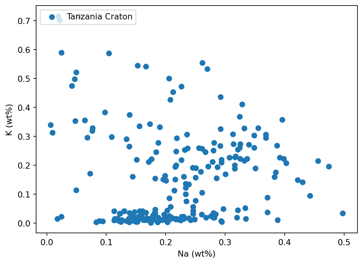

elements = ['Si', 'Ti', 'Al', 'Mg', 'Mn', 'Ni', 'Co', 'Na', 'K']

interact(pltData, xData = elements, yData = elements)

<function __main__.pltData(xData, yData)>

What’s wrong with this code? (NONE YET)

coming

Solution

coming

4.3 Command- if, elif, else [06:11]

== (›test a condition‹), True, False
Available Notebooks: Lecture, Exercise, Solution

Oftmals sollen unterschiedliche Dinge ausgeführt oder dargestellt werden, je nachdem was für eine Bedingung erfüllt ist. Wird etwa ein bestimmter Messwert unterschritten (die Bedingung), kann als Ausgabe erfolgen ›below detection limit‹. Eine Bedingung kann auch der Input eines Anwenders sein, der z.B. auswählen kann, ob auf der x-Achse die Einheit in wt% oder wt-ppm dargestellt werden soll. Bedingungen sind sehr häufig, und dieser Befehl entsprechend wichtig.

Video nb

a = 4    # assign a value to variable a
a == 4   # test a condition

True

b = 'hello'
b == 'helo'

False

mgo = 12

if mgo > 54:
    print('olivine')
elif mgo <= 54 & mgo >40:
    print('pyroxene')
else:
    print('not olivine')

not olivine

scale = 'log'

if scale == 'linear':
    print('linear scaling')
else:
    print('log scaling')

log scaling

Describe the basic concept of if/elif/else.

These are conditions, i.e., a condition is checked (e.g., if a variable is larger, smaller or equal to a certain value, or, whehter a variable has True/False as its value), and depending on whether the condition is True or False, either an output is created, or an additional condition is checked using elif.

What is the result of the following code:

mg = 22.13

if mg < 0.03
    print('below d.l.')
else:
    print(mg)

✓22.13

✗below d.l.

✗code is incomplete

✗Nothing particular

The if/elif/else command can be used with interactive elements.

✓True

✗False

Practise

An interactive plot has the opiton of ticking whether wt% or wt-ppm is shown on an axis. The value from the tick box is either True or False. In case of True, the output shall be wt%.
In the first step, we do not want a plot, but only the output of either ‘wt%’ or ‘wt-ppm’.
Make the simplest plot possible using the provided data, but depending on the value of unit, display ‘wt%’ or ‘wt-ppm’ on the y-axis.
Expand the unit selection on the previous plot by the following two options: ‘wt-ppb’ and ‘wt-ppt’.
This is challenging, as you cant use True/False any longer.
If you want to go one step further, try and combine this with interact. It is a challenge, and not yet expected to be solved.

Solution

unit = True

if unit == True:  # this needs to be '==' as no value is assigned, but test is performed.
    print('wt%')
else:
    print('wt-ppm')

wt%

import matplotlib.pyplot as plt

data = [1, 5, 2, 5, 6]

unit = True

if unit == True:  # this needs to be '==' as no value is assigned, but test is performed.
    plotUnit = '( wt%)'
else:
    plotUnit = ' (wt-ppm)'

plt.plot(data)
plt.ylabel('MgO' + plotUnit)

plt.show()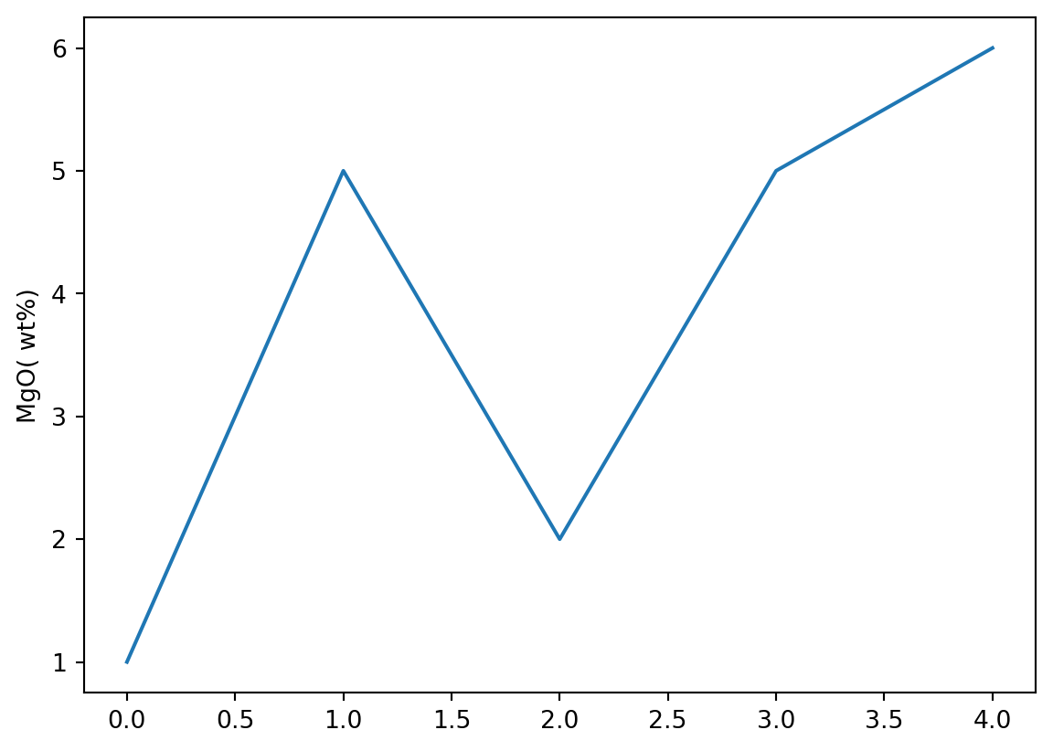

data = [1, 5, 2, 5, 6]

unit = 2

if unit == 1:  # this needs to be '==' as no value is assigned, but test is performed.
    plotUnit = '( wt%)'

elif unit == 2:
    plotUnit = ' (wt-ppm)'

elif unit == 3:
    plotUnit = ' (wt-ppb)'

else:
    plotUnit = ' (wt-ppt)'

plt.plot(data)
plt.ylabel('MgO' + plotUnit)

plt.show()

from ipywidgets import interact

def pltData(unit):
    if unit == 1:  # this needs to be '==' as no value is assigned, but test is performed.
        plotUnit = '( wt%)'
    elif unit == 2:
        plotUnit = ' (wt-ppm)'
    elif unit == 3:
        plotUnit = ' (wt-ppb)'
    else:
        plotUnit = ' (wt-ppt)'

    plt.plot(data)
    plt.ylabel('MgO' + plotUnit)

    return plt.show()

data = [1, 5, 2, 5, 6]

interact(pltData, unit = [1, 2, 3, 4])

<function __main__.pltData(unit)>

What’s wrong with this code? (NONE YET)

coming

Solution

coming

4.4 Program- Visualising data from various databases [14:47]

Available Notebooks: Lecture, Exercise, Solution

Nun wollen wir einmal möglichst viel des bisher Gelernten anwenden und um schickes Programm zu bauen, mit dem auf verschiedene Datenbanken zugreifen und deren Inhalt wie gewünscht – also Element aussuchen, Einheit festlegen – darstellen können.

Video nb

import mag4 as mg
import pandas as pd
import matplotlib.pyplot as plt
from ipywidgets import interact, widgets

def pltData(locality, x_data, y_data, x_ppm, y_ppm):
    
    df = mg.get_data(locality)

    if x_ppm == True:
        plt.xlabel(x_data + ' (wt-ppm)')
        xConv = 1
    else:
        plt.xlabel(x_data + ' (wt-%)')
        xConv = .00001
        
    if y_ppm == True:
        plt.ylabel(y_data + ' (wt-ppm)')
        yConv = 1
    else:
        plt.ylabel(y_data + ' (wt-%)')
        yConv = .00001
    
    plt.scatter(df[x_data] * xConv, df[y_data] * yConv, label = locality)
    
    plt.legend(loc = 'lower right')
    
    return plt.show()

elements = ['Si', 'Mg', 'Al', 'Na', 'Eu']
localities = ['Bastar Craton', 'West African Craton', 'Tanzania Craton Archean']

interact(pltData, locality = localities, x_data = elements, y_data=widgets.Dropdown(options=elements, value='Mg'), x_ppm = False, y_ppm = False)

<function __main__.pltData(locality, x_data, y_data, x_ppm, y_ppm)>

What is the simplest way to populate a drop-down menu?

Using a list that contains all the elements that shall be shown in this menu.

How many interacitve elements can be displayed when using interact?

✗5

✗10

✓unlimited

What is commonly the last line in a self-defined command?

✓return

✗output

✗res

✗result

Practise

Import what is needed for an interactive plot.
Code an interactive plot that allows to select and display one of the selected databases as a simple (or more sophisticated, should you wish) plot.

Then, for a real challenge:
Adjust the code so that you can choose which databases are shown – but so that they ar shown together, not individually.

Solution

import mag4 as mg
import pandas as pd
import matplotlib.pyplot as plt
from ipywidgets import interact

localities = ['Bastar Craton', 'West African Craton', 'Tanzania Craton Archean']

def pltData(locality, xData, yData):
    df = mg.get_data(locality)
    plt.scatter(df[xData] * .00001, df[yData] * .00001)
    plt.xlabel(xData + ' (wt%)')
    plt.ylabel(yData + ' (wt%)')
    return plt.show()

elements = ['Mg', 'Si', 'Al', 'Na', 'Eu']

interact(pltData, locality = localities, xData = elements, yData = elements)

<function __main__.pltData(locality, xData, yData)>

# I will now use pltData2 instead of pltData

def pltData2(bastar, westAfrican, tanzania, xData, yData):
    if bastar == True:
        dfBastar = mg.get_data(locality)
        plt.scatter(dfBastar[xData] * .00001, dfBastar[yData] * .00001, label = 'Bastar')
        
    if westAfrican == True:
        dfWestAfrican = mg.get_data(locality)
        plt.scatter(dfWestAfrican[xData] * .00001, dfWestAfrican[yData] * .00001, label = 'West African')
        
    if tanzania == True:
        dfTanzania = mg.get_data(locality)
        plt.scatter(dfTanzania[xData] * .00001, dfTanzania[yData] * .00001, label = 'Tanzania')
    
    plt.xlabel(xData + ' (wt%)')
    plt.ylabel(yData + ' (wt%)')
    plt.legend(loc = 'upper right')
    
    return plt.show()

elements = ['Mg', 'Si', 'Al', 'Na', 'Eu']

interact(pltData2, bastar = True, westAfrican = False, tanzania = False, xData = elements, yData = elements)

<function __main__.pltData2(bastar, westAfrican, tanzania, xData, yData)>

That shall be enough. But, of course, as there are 3 similar ‘if’ statements in the code, this can be made more compact. Another time.

What’s wrong with this code? (NONE YET)

coming

Solution

coming

4.5 Task- Plotting normalised REE from a database [06:15]

.pop(), .dropna(), .T, .yscale(log)
Available Notebooks: Solution

Seit einiger Zeit sollte klar werden, dass das bisher Gelernte mit den üblichen Programmen zur Analyse und Darstellung von Daten immer schwieriger würde, vor allem wenn schnell und flexibel gestaltet werden soll. Und natürlich ist das erst der Anfang. In dieser Aufgabe sollst Du erfahren, wie sehr wir uns bald auf die Ergebnisse, und weniger auf den Weg dahin konzentrieren können. Im Video werden ein paar Sachen dargestellt, dann sollst Du selbst versuchen, den unten gezeigten Plot normiert, bzw. nicht normiert darzustellen, d.h., das Programm dafür zu schreiben.

Solution

import mag4 as mg
import pandas as pd
import matplotlib.pyplot as plt
from ipywidgets import interact

df = mg.get_data('West African Craton')
dfChondrites = mg.get_data("Chondrite Element Abundances")
dfChondrites

	z	symbol	unit	CI	solar abundance	CM	CV	CO	CK	CR	CH	H	L	LL	EH	EL	R	K
0	1	H	wt%	2.02	2.880000e+10	1.40	0.28	0.07	NaN	NaN	NaN	NaN	NaN	NaN	NaN	NaN	NaN	NaN
1	2	He	NaN	NaN	2.290000e+09	NaN	NaN	NaN	NaN	NaN	NaN	NaN	NaN	NaN	NaN	NaN	NaN	NaN
2	3	Li	ppm	1.50	5.547000e+01	1.50	1.70	1.80	1.4	NaN	NaN	NaN	NaN	NaN	NaN	NaN	NaN	NaN
3	4	Be	ppm	0.03	7.370000e-01	0.04	0.05	NaN	NaN	NaN	NaN	NaN	NaN	NaN	NaN	NaN	NaN	NaN
4	5	B	ppm	0.87	1.732000e+01	0.48	0.30	NaN	NaN	NaN	NaN	NaN	NaN	NaN	NaN	NaN	NaN	NaN
...	...	...	...	...	...	...	...	...	...	...	...	...	...	...	...	...	...	...
82	83	Bi	ppb	110.00	1.388000e-01	71.00	54.00	35.00	20.0	40.0	NaN	NaN	NaN	NaN	NaN	NaN	NaN	NaN
83	89	Ac	NaN	NaN	NaN	NaN	NaN	NaN	NaN	NaN	NaN	NaN	NaN	NaN	NaN	NaN	NaN	NaN
84	90	Th	ppb	29.00	NaN	41.00	58.00	80.00	58.0	42.0	NaN	NaN	NaN	NaN	NaN	NaN	NaN	NaN
85	91	Pa	NaN	NaN	NaN	NaN	NaN	NaN	NaN	NaN	NaN	NaN	NaN	NaN	NaN	NaN	NaN	NaN
86	92	U	ppb	8.00	NaN	12.00	17.00	18.00	15.0	13.0	NaN	NaN	NaN	NaN	NaN	NaN	NaN	NaN

87 rows × 18 columns

cIValues = dfChondrites.iloc[56:71, 3].tolist()
cIValues.pop(4)  # removes Pm
cIValues

[0.235,
 0.62,
 0.094,
 0.46,
 0.15,
 0.057,
 0.2,
 0.037,
 0.25,
 0.056,
 0.16,
 0.025,
 0.16,
 0.025]

ree = ['La', 'Ce', 'Pr', 'Nd', 'Sm', 'Eu', 'Gd', 'Tb', 'Dy', 'Ho', 'Er', 'Tm', 'Yb', 'Lu']

fil = df['Rock Type'] == 'VOLCANIC ROCK'

def plotREE(normalised):
    global data
    if normalised == True:
        data = df.loc[fil, ree].dropna(axis=0, how='all') / cIValues   # .dropna() deletes all rows with no values
        plt.ylabel('normalised abundances (mass-ratios)')
    else:
        data = df.loc[fil, ree].dropna(axis=0, how='all')
        plt.ylabel('concentrations (wt-ppm)')

    plt.plot(data.T)  # .T transposes the data
    plt.yscale('log')

    return plt.show()

interact(plotREE, normalised = True)

This cell is currently not evaluated, as it causes quarto to hang for yet unknown reasons, but it should work in a jupyter notebook just fine.