[1, 2, 3, 4, 5][1, 2, 3, 4, 5]“Eine besonders effektive und interessante Art auf Daten zuzugreifen ist über ›Application Programming Interfaces‹ – kurz: API. Der Begriff API ist sehr weit verbreitet, und sollte man sich in jedem Fall merken. In einer idealen Welt hätte man gar keine eigenen Datenbanken mehr, sondern würde nur noch über APIs auf Datenbanken zugreifen, sich die gewünschten Daten herunter laden, und diese dann auf dem eigenen Computer auswerten. Ein Großteil des Internets, und viele der erfolgreichsten Apps auf dem Smartphone funktionieren genau so: über ein API werden die gewünschten Daten geladen, und die App macht letztlich nicht mehr als ein Interface zur verfügung zu stellen, um diese Daten entsprechend auszuwählen und darzustellen. Das Interface ist dabei ein Graphical User Interface – kurz GUI. Ebenfalls ein Begriff, den man kennen sollte. Eine GUI ist letztlich nichts anders als das, was wir mit ›Interact‹ kennen gelernt haben. D.h., mit einer API und einer GUI machen wir exakt das, was fast jede unserer App auf dem Smartphone macht. Das hört sich alles großartig an – und ist es auch! Wäre da nicht das eine Problem: viele geowissenschaftliche Datenbanken haben – noch – keine vernünftige API. Glücklicherweise ändert sich daran gerade viel. Fun Fact Wir hier in Frankfurt sind an dieser Änderung recht zentral beteiligt.”
Um 2000 herum begannen ein paar erste Initiativen damit mineralogische Datenbanken aufzubauen. Zu den Pionieren gehören sicherlich die GeoROC Datenbank am Max-Planck Institut für Geochemie in Mainz, die EarthChem Datenbank am Lamont-Doherty Earth Observatory, sowie die MetBase, welche von einem privaten Enthusiasten aufgebaut wurde. Die ersten beiden Datenbanken enthalten primär Gesteinsdaten, sind also geochemisch orientiert, wohingegen die MetBase eine kosmoschemische Datenbank mit Meteoriten-Daten ist. Zusätzlich gibt es Konsortien (NFDI4Earth, Research Data Alliance, European Open Science Cloud (EOSC), die selbst keine Datenbanken betreiben, sondern Standards, Schnittstellen, etc. definieren, und einen zentralen Zugangspunkt zu den verschiedenen Datenbanken anbieten. Das gibt es außerdem nicht nur für Daten, sondern auch für Labore (EPOS) oder die Lehre.
{ } (-> Dictionary brackets), pd.DataFrame()
Available Notebooks: Lecture, Exercise, Solution
Daten, die man sich aus online-Datenbanken zieht sind häufig in Listen des Typs Dictionary (z.B. json Formate). Dictionary sind schnell zugänglich und leicht verständlich nachdem wir nun Pandas DataFrames kenne – und können auch direkt in diese umformatiert werden.
requests, .get(), json, str()
Available Notebooks: Lecture, Exercise, Solution
Was ist eine API? Ein Application Programming Interface. Das sagt kaum mehr. Es ist eine Schnittstelle. Hilft vielleicht etwas. Angenommen, wir wollen die aktuellen Wetterdaten einer Stadt wissen. Dann können wir eine Anfrage (request) an einen Server stellen, und bekommen die Wetterdaten geliefert. Hört sich einfach an – und ist es tatsächlich auch. In dieser Einheit lernen wir also, wie wir sehr einfach Daten von einem Server in unser Jupyter Notebook laden, und dort darstellen, weiter verarbeiten, visualisieren, etc. können.
~filter, .isin(), .str.contains(), .index, .value_count(), .rename, export, .to_csv, .to_excel
In dieser zweiten Einheit zu Pandas lernen wir weitere Möglichkeiten um Daten in pandas dataframes zu manipulieren, zählen, exportieren, etc. Es macht jedoch keinen Sinn, in diesem Kurs den vollständigen Umfang von Pandas – oder jeglicher anderer Python-Bibliothek – darzustellen. Vielmehr sucht man sich je nach zu lösender Fragestellung die nötigen Befehle aus dem persönlichen Fundus plus der entsprechenden Recherche in den einschlägigen Ressourcen aus dem Internet zusammen.
Exercises are in preparation
Available Notebooks: Lecture, Exercise, Solution
Zum Abschluss der Einheit wollen wir ein konkretes Beispiel für Data Science anschauen. Die Eu- Anomalie kennen vermutlich alle – sonst schnell mal nachschauen, was das ist. Wie sie berechnet wird, wird jedoch im Video erklärt. Am Ende werden wir ein sehr kurzes Programm haben, mit dem sich (i) die Eu-Anomalie analysieren lässt, und das (ii) sehr flexibel ist, d.h. mit dem wir nun prinzipiell die Eu-Anomalie jeder beliebigen Datenbank analysieren können.
Import libraries and read the file
import pandas as pd
import matplotlib.pyplot as plt
import mag4 as mg
df = mg.get_data('Tanzania Craton Archean')Data selection and clean-up
*Be aware that the syntax for the dropna() argument changed. Instead of dropna(0) it is now dropna(axis=0).
cISmEuGd = [.15, .057, .2]

smEuGdData = df.loc[:, ['Sm', 'Eu', 'Gd']].dropna(axis=0) / cISmEuGd

smEuGdData| Sm | Eu | Gd | |
|---|---|---|---|
| 11 | 34.600000 | 25.789474 | 21.10 |
| 12 | 28.066667 | 19.649123 | 19.80 |
| 13 | 41.933333 | 29.473684 | 27.35 |
| 14 | 49.266667 | 32.280702 | 30.60 |
| 15 | 26.800000 | 20.526316 | 18.50 |
| ... | ... | ... | ... |
| 230 | 49.200000 | 33.508772 | 28.60 |
| 231 | 54.200000 | 37.017544 | 28.55 |
| 232 | 52.400000 | 34.035088 | 29.15 |
| 233 | 47.800000 | 30.877193 | 27.25 |
| 234 | 45.333333 | 28.947368 | 25.55 |
206 rows × 3 columns
len(smEuGdData)206Calculate the anomaly and convert to a pandas dataframe
res = []

for n in range(len(smEuGdData)):
    l = smEuGdData.iloc[n].tolist()
    euAn = ((l[1] / ((l[0] + l[2]) / 2)) - 1) * 100
    res.append(round(euAn))


res
[-7,
-18,
-15,
-19,
-9,
-9,
-17,
-11,
-12,
-4,
-10,
-3,
-15,
-9,
-8,
-15,
-12,
-10,
-17,
-11,
-14,
-10,
0,
-11,
-15,
-10,
-17,
-21,
-7,
-15,
-12,
-8,
-13,
-12,
-10,
-18,
-19,
-14,
-10,
-22,
-22,
-17,
1,
1,
-60,
0,
-3,
5,
-4,
-9,
1,
1,
0,
6,
0,
7,
11,
-14,
-3,
-3,
0,
-1,
5,
-7,
-5,
13,
1,
-6,
-3,
1,
14,
-20,
14,
42,
0,
7,
-19,
58,
8,
6,
7,
3,
-8,
8,
-16,
7,
22,
-2,
0,
35,
3,
10,
-31,
-29,
-15,
-11,
-7,
-5,
-3,
-7,
13,
12,
-6,
-7,
-2,
3,
1,
3,
0,
-3,
-25,
-36,
-4,
-9,
-38,
-33,
-38,
-14,
-41,
-29,
-24,
-36,
-26,
-21,
-9,
-32,
-48,
-22,
-15,
-35,
-43,
-20,
22,
-19,
-27,
-10,
-11,
-1,
-92,
-98,
-98,
-83,
6,
-2,
6,
-2,
17,
7,
0,
8,
8,
-1,
12,
-2,
3,
3,
-1,
-12,
-4,
23,
9,
7,
12,
-3,
18,
19,
20,
4,
6,
1,
3,
13,
-10,
-5,
14,
-25,
-34,
-56,
-44,
9,
-73,
-70,
-52,
-38,
-25,
-31,
-54,
-33,
-42,
-68,
-11,
-48,
-12,
-20,
-33,
-48,
-54,
-52,
-59,
-13,
-8,
-14,
-11,
-17,
-18,
-18]Visualise the data
plt.plot(res)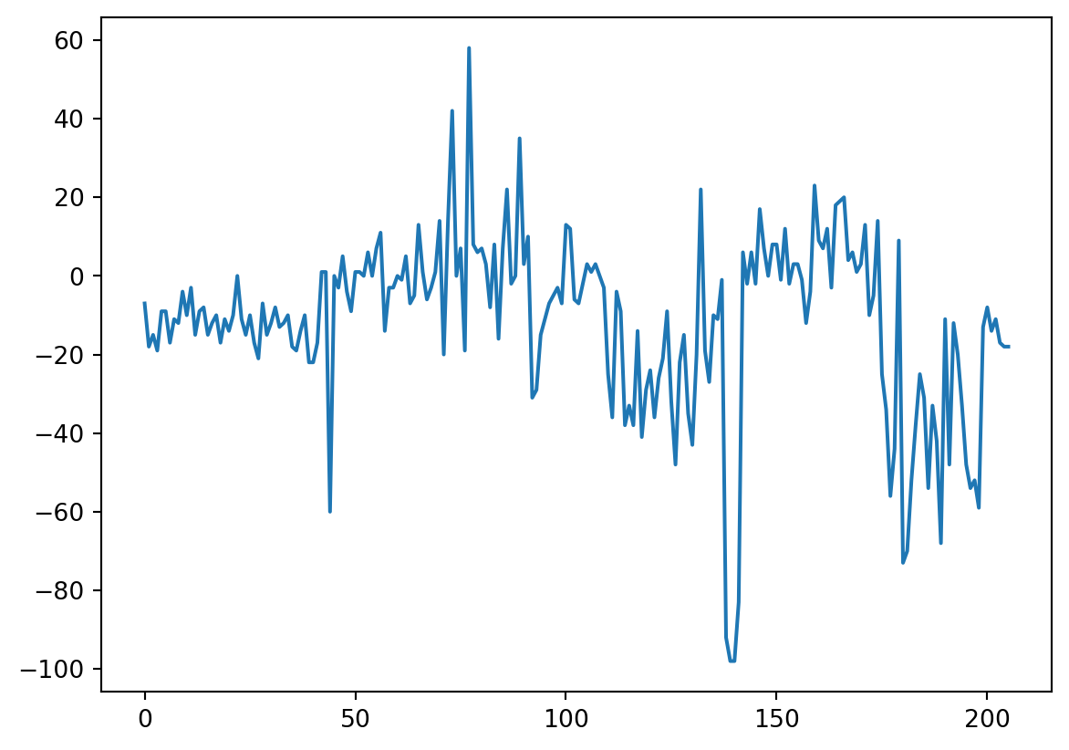
All in one (or at least the last 3 parts in one)
cISmEuGd = [.15, .057, .2]
smEuGdData = df.loc[:, ['Sm', 'Eu', 'Gd']].dropna(axis=0) / cISmEuGd

res = []

for n in range(len(smEuGdData)):
    l = smEuGdData.iloc[n].tolist()
    euAn = ((l[1] / ((l[0] + l[2]) / 2)) - 1) * 100
    res.append(round(euAn))

plt.plot(res)
plt.show()
We now want to calculate the anomaly of every REE element.
The element of interest shall be selectable from a drop-down menu.
Start with importing the required libraries and/or commands. Below we will ned the REE CI concentrations. Start with extracting these.
To do this, read in the CI data from 'Chondrite Element Abundances' using mag4 into the variable ‘cIdf’.
Define a command to find the index of a specific element.
(Maybe store this handy posRow() command in your 'mineralogyModule.py'.)
Use this command to select only the datasates with the SEE.
Extract the CI REE (-> from La to Lu) concentrations as a list from the imported chondrite element abundances file. Make sure you extracted the correct values.
Delete Pm from this list.
Below follows the program from the corresponding unit. Convert this program into a command called 'calcREEAnomaly'. Input to the command shall only be the REE element for which the anomlay shall be calculated, and the dataset, for which the anomaly shall be calculated.
As this is not trivial, you might want to have a peak at the solution.
As we only have the REE for which the anomaly shall be calculated, we first need modify the program to accomodate for this.
First, produce a list of the names of the REE without Pm.
Using the input REE, produce the list of the 3 REE called ‘threeREE’ required for calculating the anomaly.
You can then do the same with the cIREE list, i.e., selcet the REE values for these elements.
Then modify the program above:
(i) so that the 3 REE are now automaticall chosen depending on the single REE input.
(ii) so that the 3 REE CI concentrations are now automaticall chosen depending on the single REE input.
Finally you can convert this program into the command 'calcREEAnomaly' that calculates the anomaly of every REE (except for two, do you know which?), depending on user input.
Read in the 'West African Cratons' dataset as df.
Finally test your freshly defined command with e.g., calcREEAnomaly('Eu').
Expand your command so it displays a graph rather than a list of values.
Test wheter it works.
‘mineralogyModule’. (Maybe add this command to your 'mineralogyModule.py'.)
And for easier usage, make it interactive, where you can choose the element from a drop-down menu – that displays only thos elements, for which anomalies can be calculated.
(You might occassionally get an error, don’t worry, just try another element. Most should work. The error is most likely because of some missing or zero values. These could be avoided with accoriding ‘if’ statements and some kind of informative message.)
import pandas as pdBe aware that the key is no longer 'Element', but 'symbol'
cIdf = mg.get_data('Chondrite Element Abundances')

def posRow(name):
return cIdf.index[cIdf['symbol'] == name][0]cIdf.loc[posRow('La'):posRow('Lu')]| z | symbol | unit | CI | solar abundance | CM | CV | CO | CK | CR | CH | H | L | LL | EH | EL | R | K | |
|---|---|---|---|---|---|---|---|---|---|---|---|---|---|---|---|---|---|---|
| 56 | 57 | La | ppm | 0.235 | 0.44200 | 0.320 | 0.469 | 0.380 | 0.460 | 0.310 | 0.290 | 0.301 | 0.318 | 0.330 | 0.240 | 0.196 | 0.310 | 0.320 |
| 57 | 58 | Ce | ppm | 0.620 | 1.19100 | 0.940 | 1.190 | 1.140 | 1.270 | 0.750 | 0.870 | 0.763 | 0.970 | 0.880 | 0.650 | 0.580 | 0.830 | NaN |
| 58 | 59 | Pr | ppm | 0.094 | 0.17310 | 0.137 | 0.174 | 0.140 | NaN | NaN | NaN | 0.120 | 0.140 | 0.130 | 0.100 | 0.070 | NaN | NaN |
| 59 | 60 | Nd | ppm | 0.460 | 0.83550 | 0.626 | 0.919 | 0.850 | 0.990 | 0.790 | NaN | 0.581 | 0.700 | 0.650 | 0.440 | 0.370 | NaN | NaN |
| 60 | 61 | Pm | NaN | NaN | NaN | NaN | NaN | NaN | NaN | NaN | NaN | NaN | NaN | NaN | NaN | NaN | NaN | NaN |
| 61 | 62 | Sm | ppm | 0.150 | 0.25420 | 0.204 | 0.294 | 0.250 | 0.290 | 0.230 | 0.185 | 0.194 | 0.203 | 0.205 | 0.140 | 0.149 | 0.180 | 0.200 |
| 62 | 63 | Eu | ppm | 0.057 | 0.09599 | 0.078 | 0.105 | 0.096 | 0.110 | 0.080 | 0.076 | 0.074 | 0.080 | 0.078 | 0.052 | 0.054 | 0.072 | 0.080 |
| 63 | 64 | Gd | ppm | 0.200 | 0.33880 | 0.290 | 0.405 | 0.390 | 0.440 | 0.320 | 0.290 | 0.275 | 0.317 | 0.290 | 0.210 | 0.196 | NaN | NaN |
| 64 | 65 | Tb | ppm | 0.037 | 0.05701 | 0.051 | 0.071 | 0.060 | NaN | 0.050 | 0.050 | 0.049 | 0.059 | 0.054 | 0.034 | 0.032 | NaN | NaN |
| 65 | 66 | Dy | ppm | 0.250 | 0.39220 | 0.332 | 0.454 | 0.420 | 0.490 | 0.280 | 0.310 | 0.305 | 0.372 | 0.360 | 0.230 | 0.245 | 0.029 | NaN |
| 66 | 67 | Ho | ppm | 0.056 | 0.08666 | 0.077 | 0.097 | 0.096 | 0.100 | 0.100 | 0.070 | 0.074 | 0.089 | 0.082 | 0.050 | 0.051 | 0.059 | NaN |
| 67 | 68 | Er | ppm | 0.160 | 0.25040 | 0.221 | 0.277 | 0.305 | 0.350 | NaN | NaN | 0.213 | 0.252 | 0.240 | 0.160 | 0.160 | NaN | NaN |
| 68 | 69 | Tm | ppm | 0.025 | 0.03700 | 0.035 | 0.048 | 0.040 | NaN | NaN | 0.040 | 0.033 | 0.038 | 0.035 | 0.024 | 0.023 | NaN | NaN |
| 69 | 70 | Yb | ppm | 0.160 | 0.24840 | 0.215 | 0.312 | 0.270 | 0.320 | 0.220 | 0.210 | 0.203 | 0.226 | 0.230 | 0.154 | 0.157 | 0.216 | 0.215 |
| 70 | 71 | Lu | ppm | 0.025 | 0.03738 | 0.033 | 0.046 | 0.039 | 0.046 | 0.032 | 0.030 | 0.033 | 0.034 | 0.034 | 0.025 | 0.025 | 0.032 | 0.033 |
cIREE = cIdf.loc[posRow('La'):posRow('Lu'), 'CI'].tolist()

cIREE.pop(4)

cIREE
[0.235,
0.62,
0.094,
0.46,
0.15,
0.057,
0.2,
0.037,
0.25,
0.056,
0.16,
0.025,
0.16,
0.025]cISmEuGd = [.15, .057, .2]
smEuGdData = df.loc[:, ['Sm', 'Eu', 'Gd']].dropna(axis=0) / cISmEuGd
res = []
for n in range(len(smEuGdData)):
l = smEuGdData.iloc[n].tolist()
euAn = ((l[1] / ((l[0] + l[2]) / 2)) - 1) * 100
res.append(round(euAn))Be aware that the key is no longer 'Element', but 'symbol'
ree = cIdf.loc[posRow('La'):posRow('Lu'), 'symbol'].tolist()

ree.pop(4)
ree
['La',
'Ce',
'Pr',
'Nd',
'Sm',
'Eu',
'Gd',
'Tb',
'Dy',
'Ho',
'Er',
'Tm',
'Yb',
'Lu']# input REE
el = 'Eu'
# either
leftREE = ree[ree.index(el) - 1]
rightREE =ree[ree.index(el) + 1]
threeREE = [leftREE, el, rightREE]
print(threeREE)
# or
threeREE = [ree[ree.index(el) - 1], el, ree[ree.index(el) + 1]]
print(threeREE)['Sm', 'Eu', 'Gd']
['Sm', 'Eu', 'Gd']el = 'Eu'
cISmEuGd = [cIREE[ree.index(el) - 1], cIREE[ree.index(el)], cIREE[ree.index(el) + 1]]
threeREE = [ree[ree.index(el) - 1], el, ree[ree.index(el) + 1]]
smEuGdData = df.loc[:, threeREE].dropna(axis=0) / cISmEuGd
res = []
for n in range(len(smEuGdData)):
l = smEuGdData.iloc[n].tolist()
euAn = ((l[1] / ((l[0] + l[2]) / 2)) - 1) * 100
res.append(round(euAn))def calcREEAnomaly(el):
cISmEuGd = [cIREE[ree.index(el) - 1], cIREE[ree.index(el)], cIREE[ree.index(el) + 1]]
threeREE = [ree[ree.index(el) - 1], el, ree[ree.index(el) + 1]]
smEuGdData = df.loc[:, threeREE].dropna(axis=0) / cISmEuGd
res = []
for n in range(len(smEuGdData)):
l = smEuGdData.iloc[n].tolist()
euAn = ((l[1] / ((l[0] + l[2]) / 2)) - 1) * 100
res.append(round(euAn))
return resdf = mg.get_data('West African Craton')calcREEAnomaly('Eu')[-13,
2,
6,
21,
-65,
-11,
-23,
15,
-64,
-46,
12,
-5,
13,
12,
12,
10,
0,
7,
-2,
-5,
12,
-3,
-1]import matplotlib.pyplot as pltdef calcREEAnomaly(el):
cISmEuGd = [cIREE[ree.index(el) - 1], cIREE[ree.index(el)], cIREE[ree.index(el) + 1]]
threeREE = [ree[ree.index(el) - 1], el, ree[ree.index(el) + 1]]
smEuGdData = df.loc[:, threeREE].dropna(axis=0) / cISmEuGd
res = []
for n in range(len(smEuGdData)):
l = smEuGdData.iloc[n].tolist()
euAn = ((l[1] / ((l[0] + l[2]) / 2)) - 1) * 100
res.append(round(euAn))
plt.plot(res)
return plt.show()calcREEAnomaly('Sm')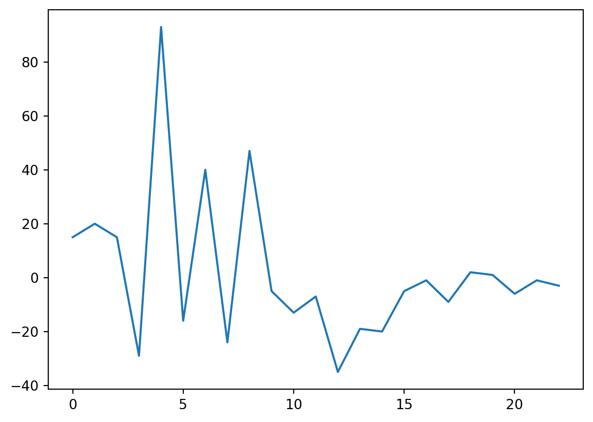
from ipywidgets import interactinteract(calcREEAnomaly, el = ['Ce', 'Pr', 'Nd', 'Sm', 'Eu', 'Gd', 'Tb', 'Dy', 'Ho', 'Er', 'Tm', 'Yb'])<function __main__.calcREEAnomaly(el)>